Polymath proposal: The Hot Spots Conjecture for Acute Triangles

June 3, 2012

Polymath proposal: The Hot Spots Conjecture for Acute Triangles

Filed under: hot spots,polymath proposals — Terence Tao @ 2:59 am

Chris Evans has proposed a new polymath project, namely to attack the “Hot Spots conjecture” for acute-angled triangles. The details and motivation of this project can be found at the above link, but this blog post can serve as a place to discuss the problem (and, if the discussion takes off, to start organising a more formal polymath project around it).

Comments (111)

111 Comments »

Some initial questions to get the ball rolling:

It seems that there are two versions of the “hot spots” conjecture in the literature:

(i) the hot spots conjecture for generic data;
(ii) the hot spots conjecture for arbitrary data.

As I understand it, (i) is equivalent to saying that a (generic) eigenfunction of the first nontrivial eigenvalue of the Laplacian (with Neumann boundary data) attains its maximum on the boundary, while (ii) is equivalent to the same claim, but for _all_ eigenfunctions and non-trivial eigenvalues. Given that (i) would be easier, I presume that this is the version of the conjecture to attack?

Also, could the conjecture be solved numerically for specific triangles, such as the equilateral triangle?

Comment by Terence Tao — June 3, 2012 @ 3:09 am | Reply
- Brian J. McCartin has recently published a book, downloadable at http://www.m-hikari.com/mccartin-3.pdf, “LAPLACIAN EIGENSTRUCTURE OF THE EQUILATERAL
  TRIANGLE”, where he states; “in 1833, Gabriel Lam´e discovered analytical formulae for the complete eigenstructure of the Laplacian on the equilateral
  triangle under either Dirichlet or Neumann boundary conditions and a portion of the corresponding eigenstructure under a Robin boundary condition. Surprisingly,
  the associated eigenfunctions are also trigonometric. The physical context for his pioneering investigation was the propagation of heat throughout polyhedral bodies.”
  
  Comment by Stuart Anderson — June 5, 2012 @ 8:42 am | Reply
  - In reply to Stuart Anderson: Brian J. McCartin also has a published paper in “Mathematical Problems in Engineering”, Vol. 8 , Issue 6, Pages 517-539, entitled: “Eigenstructure of the equilateral triangle, Part II: The Neumann problem”. There, he gives a complete description of Lame’s eigenfunctions for an
    equilateral triangle with a Neumann boundary coundition (del U)/(del n) = 0 , n the normal to the
    triangular boundary, U an eigenfuntion. In section 8 on Modal Properties, he gives beautiful
    expressions for the eigenfunctions in terms of pairs of integers (m, n) in Equations 8.1 and 8.2, where
    (8.1) covers what McCartin calls the symmetric, and (8.2) the antisymmetric modes (respectively).
    
    I’m intrigued by whether the modes in equations (8.1) and (8.2) always attain their max and min
    on the boundary of the triangular region (equilateral triangle); the 3D plots of several modes by
    McCartin seems consistent with max/min always being attained on the boundary; Lame solved
    the equilateral triangle case, in the sense that he gave a complete set of eigenfunctions for
    the Laplacian eigenvalue problem with the (del U)/(del n) = 0 boundary value condition.
    David Bernier
    
    Edit: Link to the paper is http://downloads.hindawi.com/journals/mpe/2002/591873.pdf
    
    Comment by meditationatae — June 5, 2012 @ 12:06 pm | Reply
    - I worked out the second eigenspace for the equilateral triangle and the answer is actually rather pretty. It is convenient to work in the plane $\{ (x,y,z): x+y+z=0\}$ and take the equilateral triangle spanned by (0,0,0),(1,0,-1), (1,-1,0). Then it turns out that there is a two-dimensional eigenspace for the second eigenfunction, spanned by the real and imaginary parts of the complex eigenfunction
      
      $\exp( 2\pi i(x-y) / 3 ) + \exp( 2\pi i(y-z) / 3 ) + \exp( 2\pi i(z-x) / 3 )$ .
      
      This complex eigenfunction maps the equilateral triangle to a slightly concave version of the equilateral triangle, so that whenever one takes a projection of this complex eigenfunction to create a real eigenfunction, the maximum and minimum are only attained at the corners. Because of this strict concavity it seems likely to me that this property persists with respect to small perturbations of the domain. (I think one can use the Rayleigh quotient formalism and some suitable changes of variable to show that second eigenvalues and eigenfunctions of a perturbed domain must be close to second eigenvalues and eigenfunctions of the original domain, though I’m not sure yet exactly what function space norms one can use to define closeness of eigenfunctions here.)
      
      Comment by Terence Tao — June 10, 2012 @ 3:39 am | Reply
      - I’m trying to understand how to verify the concavity of the image. If A designates the point (0,0,0) , B designates the point (1, -1, 0) and C designates the point (1, 0, -1), then a point on the edge from A to B is a convex combination tA + (1 -t)B of the vectors A, B with $0 \leq t \leq1$ . It follows that x-y = 0 on the edge from A to B. Also, z = 0 along the edge from A to B. I would redo the convex combination with parameter t in [0, 1] for the two other edges: from A to C and from B to C. If I understand you well, the image is a figure (closed subset) of the complex plane C.
        David Bernier
        
        Comment by meditationatae — June 10, 2012 @ 7:54 am | Reply
        
        Yes, this is right (except that one has x+y=0 rather than x-y=0). For instance, on the line from A to B, the complex eigenfunction traces out the curve $t \mapsto \exp(4\pi i t / 3) + 2 \exp( - 2\pi i t/3)$ for $0 \leq t \leq 1$ , which is a concave curve from 3 to $3 \exp(4 \pi i/3)$ which can be seen for instance here. The other two sides of the triangle give rotations of this arc, tracing out the concave triangle with vertices at $3, 3 \exp(2\pi i/3), 3 \exp(4\pi i/3)$ . One can show that the eigenfunction has no critical points in the interior of the triangle, so that the image is precisely the interior of the concave triangle.
        
        Comment by Terence Tao — June 10, 2012 @ 3:54 pm | Reply
Reblogged this on Guzman's Mathematics Weblog.

Comment by Luis R. Guzman, Jr. — June 3, 2012 @ 4:37 am | Reply
How about approximating the eigenfunction by polynomials? The Neumann boundary conditions already imply that the corners are critical points. Perhaps starting with that observation, for sufficiently low degree, the geometry of the triangle implies that one of them must be a max/min. In an ideal world, a 2d version of the Sturm comparison theorem (if one exists) could then show that this feature of the polynomial approximation remains true for the actual eigenfunction. Just some preliminary ideas…

Comment by Igor Khavkine — June 3, 2012 @ 2:22 pm | Reply
- I am afraid I am not familiar with the Sturm comparison theorem and so I don’t quite follow your idea. I looked briefly at the Wikipedia page on it but I can’t figure out its connection to eigenfunctions.
  
  Is there a way for example that the Sturm comparison theorem can be used to show that the second eigenfunction for the Neumann Laplacian on the interval [0,1] has its extrema at the endpoints?
  
  Comment by Chris Evans — June 3, 2012 @ 10:43 pm | Reply
  - In my understanding, Sturm-type results allow you to establish some qualitative property for solutions of an ODE (a 1d elliptic problem) provided that the desired property holds for a nearby solution of a nearby ODE. The property usually considered is the presence of a zero (node) of an eigenfunction in some interval. I think a similar result holds for critical points of eigenfunctions.
    
    Say you could establish that the second eigenfunction of the Laplacian on a right angled triangle satisfies the desired maximum principle by showing that its only critical points are at the vertices (so that whatever the maximum is, it would have to be at one of these points). Then appealing to a comparison theorem might be able to show that the same property holds for almost-right acute triangles. Mind you, this is all speculation at this point…
    
    Comment by Igor Khavkine — June 4, 2012 @ 6:52 am | Reply
    - Ah, so maybe a Sturm-type result can make rigorous the statement: “the second eigenfunction depends continuously on the domain”? By physical considerations, this statement ought to be true.
      
      But then it seems this would only work to prove the conjecture for triangles close to right triangles?
      
      As a side note, if such a continuity statement were to hold then the hot spots conjecture for acute triangles must be true by the following *non-math* proof: If it weren’t true then by continuity there would be an open set of angles where it failed to hold. But after simulating many triplets of angles the conjecture always holds. C’mon, What are the odds we missed that open set? :-)
      
      Comment by Chris Evans — June 5, 2012 @ 3:51 am | Reply
      - It appears that Sturm’s classical work has far reaching generalizations, as described for instance in this monograph: Kurt Kreith, Oscillation Theory LNM-324, (Springer, 1973). In particular, Chapter 3 features some comparison theorems for solutions to elliptic equations.
        
        Comment by Igor Khavkine — June 5, 2012 @ 1:14 pm | Reply
Although I mentioned a “combinatorial version of the conjecture” in the proposal, I didn’t write out the details there to prevent clutter. Here is a brief write up of a combinatorial approach:

http://www.math.missouri.edu/~evanslc/Polymath/Combinatorics

While in some sense this is just another side of the same coin, perhaps rephrasing the problem as a combinatorics problem may make certain aspects more clear to combinatorics professionals.

Comment by Chris Evans — June 3, 2012 @ 7:43 pm | Reply
Also, here is the MATLAB program I’ve used to generate and display the eigenvectors of the graphs $G_n$ :

http://www.math.missouri.edu/~evanslc/Polymath/HotSpotsAny.m

The input format is HotSpotsAny(n,a,b,c,e), where a,b,c are the edge weights, n is the number of rows in the graph, and e determines which eigenvector of the graph Laplacian is displayed. (Note that in the proposal write up the graph $G_n$ has $2^n$ rows so if you wanted to simulate the Fiedler vector for $G_6$ with edge weights a=1,b=2,c=3 then you would type HotSpotsAny(64,1,2,3,2)).

For large n, the eigenvectors of the graph Laplacian should approximate the eigenfunctions of the Neumann Laplacian of the corresponding triangle… so the program can be used to roughly simulate the true eigenfunctions as well.

(Also thanks to Robert Gastler of the Univ of Missouri who wrote the first version of this code)

Comment by Chris Evans — June 3, 2012 @ 8:11 pm | Reply
Just as a loose comment: maybe ideas based on self-similarity of the whole triangle to its 4 pieces can help (i.e. modeling the whole triangle as its scaled copies + the heat contact). Then without going into the graph approximation (which looks fruitful anyway), one can see some properties.

Comment by pmigdal — June 4, 2012 @ 1:37 pm | Reply
- One advantage in the graph case is that after dividing and dividing the triangles you get to the graph $G_1$ which is simply a tree of four nodes and there I think the theorem shouldn’t be too hard to prove. And from there there might be an argument by induction. In the continuous case, no matter how many times you subdivide the triangle, after zooming it it is still the same triangle.
  
  On the other hand, in the continuous case, each of the sub-triangles is truly the same as the larger triangle. So you may be right that there is something to exploit there. Does anyone know of good examples where self-similarity techniques are used to solve a problem?
  
  In either case, there is the issue that while the biggest triangle has Neumann boundaries, the interior subtriangles have non-Neumann boundaries…
  
  Comment by Chris Evans — June 5, 2012 @ 3:39 am | Reply
- Something that is true and uses that the whole triangle is the union of the 4 congruent pieces is the following. From each eigenfunction of the triangle with eigenvalue lambda we can build another eigenfunction with eigenvalue 4 lambda by scaling the triangle to half length, and then using even reflection through the edges. Note that this eigenfunction will have an interior maximum since every point on the boundary has a corresponding point inside (on the boundary of the triangle in the middle).
  
  I’m skeptical this observation could be of any use.
  
  Comment by Luis S — June 7, 2012 @ 10:10 am | Reply
  - Hmm… but, apart from the case of an equilateral triangle, when you divide a triangle into four sub-triangles, I don’t believe that the sub-triangles are reflections of one another.
    
    Comment by Chris Evans — June 7, 2012 @ 5:43 pm | Reply
    - You’re right. My bad.
      
      Comment by Luis S — June 10, 2012 @ 1:35 am | Reply
[…] polymath related items for this post. Firstly, there is a new polymath proposal over at the polymath blog, proposing to attack the “hot spots conjecture” (concerning a maximum principle for a […]

Pingback by Two polymath projects « What’s new — June 5, 2012 @ 12:44 am | Reply
In the case of an equilateral triangle, for the Hot Spots Conjecture to hold, the second eigenvalue must, by a symmetry argument, have multiplicity at least two. The refined conjecture calls for a simple eigenvalue in the scalene case, and eigenfunction extremes at the two smaller angles. Has anyone done numerical work yet to estimate how sensitive the eigenvalue degeneracy lifting is to perturbations of a starting equilateral triangle? Any proof will have to address the issue that the third eigenvalue may be arbitrarily close to the second and has an eigenfunction with extremes at a different pair of corners.

Comment by Tracy Hall — June 5, 2012 @ 2:45 am | Reply
- Here is some preliminary data. As I am not sure how to simulate the true eigenfunctions of the triangle, the following is for the graph $G_6$ whose eigenvectors should roughly approximate the true eigenfunctions:
  
  For the case that a=b=c=1 (Equilateral Triangle):
  HotSpotsAny(64,1,1,1,2) yields the corresponding eigenvalue -0.001070825047269
  HotSpotsAny(64,1,1,1,3) yields the corresponding eigenvalue -0.001070825047269
  HotSpotsAny(64,1,1,1,4) yields the corresponding eigenvalue -0.003211901603854
  
  We see that indeed the eigenvalue -0.001070825047269 has multiplicity two.
  
  Perturbing a slightly we have that for a=1.1, b = 1, c = 1 (Isosceles Triangle where the odd angle is larger than the other two):
  HotSpotsAny(64,1.1,1,1,2) yields the corresponding eigenvalue -0.001078552707489
  HotSpotsAny(64,1.1,1,1,3) yields the corresponding eigenvalue -0.001131412869938
  
  Whereas for a=.9, b = 1, c = 1 (Isosceles Triangle where the odd angle is smaller than the other two):
  HotSpotsAny(64,.9,1,1,2) yields the corresponding eigenvalue -0.001004876221957
  HotSpotsAny(64,.9,1,1,3) yields the corresponding eigenvalue -0.001062028119964
  
  In either case we see that the third eigenvalue is perturbed away from the second.
  
  What strikes me as interesting is how different the outcome is in increasing a by 0.1 versus decreasing a by 0.1. In the former case, the second eigenvalue barely changes whereas in the latter case the second eigenvalue changes quite a bit. I imagine this ties into the heuristic “sharp corners insulate heat” — reducing a to .9 produces a sharper corner leading to more heat insulation and a much smaller (in absolute value) second eigenvalue, whereas increasing a to 1.1 makes that corner less sharp but the other two corners are still relatively sharp so the heat insulation isn’t affected as much. Just a guess though…
  
  Comment by Chris Evans — June 5, 2012 @ 4:49 am | Reply
  - It looks like the degeneracy lifting might be linear. It’s the ratio of the second and third eigenvalues that matters more, which is close to the same in either case, and approximately half as far from 1 as the perturbation. Using (9/10, 1, 1) should be the same as using (1, 10/9, 10/9) and then scaling all eigenvalues by 90%.
    
    Comment by Tracy Hall — June 5, 2012 @ 5:38 am | Reply
If the sides of the triangle have lengths A, B, and C, currently you are using edge weights a=A, b=B, and c=C. This solves a different heat equation, when you pass to the limit, than the one you want. The assumption that each small triangle is at a uniform temperature gives an extra boost to the overall heat conduction rate in those directions along which the small triangles are longer, so in the limit you are modeling heat conduction in a medium with anisotropic thermal properties. It is just as though you started with a material of extremely high thermal conductivity and then sliced it in three different directions, with three different spacings, to insert thin strips of insulating material of a constant thickness.

Based on some edge cases, I suspect that the correct formulas for edge weights to model an isotropic material in the limit are as follows: $a = 1/(-A^2+B^2+C^2)$ , $b=1/(A^2-B^2+C^2)$ , $c=1/(A^2+B^2-C^2)$ . Interestingly enough, these formulas are only defined (with positive weights) in the case of acute triangles, which suggests that this approach, if it works, may not provide an independent proof of the known cases.

Comment by Tracy Hall — June 5, 2012 @ 8:45 am | Reply
- An excellent point… it may therefore be that the $G_n$ don’t converge to the true triangle at all. And it would show that naive physical intuition might lead one astray…
  
  It might be interesting to see what the $G_n$ do converge to… if they converge at all (though remember if we want to look at converegence, we have to divide a,b, and c by two every time we increase n by one as the triangles halve in length each iteration). If they converge to a “dilated” Laplacian then maybe one could stretch the triangle to stretch it back into a Normal Laplacian (and therefore prove the conjecture for this stretched triangle).
  
  This then goes back to what you mentioned: What is the true relation between the side lengths of the triangle A,B, and C and the graph weights a, b, c.
  
  Where did you get the relations $a = 1/(-A^2+B^2+C^2), b=1/(A^2-B^2+C^2), c=1/(A^2+B^2-C^2)$ from?
  
  One last thing: I am still not convinced that the $G_n$ shouldn’t converge to the correct triangle (i.e. a=A,b=B,c=C). While its true that the heat-flow is anisotropic in the graphs (and hence their limit), the graphs $G_n$ are structurally equilateral in the “spacing of the nodes”. That is, maybe the $G_n$ converge to an *equilateral* triangle with anisotropic heat flow… which then would be equivalent to the usual heatflow on a scalene triangle?
  
  Comment by Chris Evans — June 6, 2012 @ 12:21 am | Reply
  - Running the data for a=1, b = 1.5, c = 2
    
    HotSpotsAny(2^n,1*(.5)^n,1.5*(.5)^n,2*(.5)^n,2) for n=1,…,6 yields:
    
    n=1 yields the second eigenvalue as -0.567396047577611
    n=2 yields the second eigenvalue as -0.079407110995481
    n=3 yields the second eigenvalue as -0.010175074142110
    n=4 yields the second eigenvalue as -0.001279605383718
    n=5 yields the second eigenvalue as -0.0001601915458021453
    n=6 yields the second eigenvalue as -0.00002003146751408886
    
    So it seems that the second eigenvalue of the graphs $G_n$ isn’t converging (to the true Laplacian or any dialated Laplacian for that matter)… which is disappointing. Perhaps the scaling factor of 1/2 is wrong… or perhaps the $G_n$ fail to model any diffusion on the triangle…
    
    Or it could be that n needs to be larger to see convergence… my MATLAB refuses to run n=7 so that’s as far as I could go.
    
    Comment by Chris Evans — June 6, 2012 @ 12:59 am | Reply
  - There is a PDEToolbox in MATLAB, that can find numerically (finite elements) eigenvalues and eigenfunctions for just about any domain in 2D. One can draw a domain, set Neumann boundary conditions, refine a mesh and solve.
    
    There is also a Python package called FEniCS (also finite elements), which can handle 2D and 3D. I was working on Laplace eigensolver using this package. I might be able to post something soon. Any triangle I have tried gives maximum and minimum for the second eigenfunction in the vertices connected by the longest side.
    
    Comment by Bartlomiej Siudeja — June 12, 2012 @ 5:53 pm | Reply
    - Indeed, and Matlab’s FEM package is what I used to generate the first few examples. The devil, as with any numerical algorithm, is in the details. The PDEtoolbox uses piecewise linears, and the eigenvalue solve is through an Arnoldi iteration. You’re restricting in how fine the mesh can be (due to memory management). You will see convergence, but have no real control on the asymptotic constant.
      
      Both deal.ii and FreeFem allow for higher order approximation, and more control over the numerical linear algebra. And both are freewares.
      
      Comment by Nilima Nigam — June 12, 2012 @ 5:56 pm | Reply
      - FEnics package can also use arbitrary degree for the mesh. But I agree, eventually you run into not enough memory problem. I was implementing adaptive refinements based on the second eigenfunction and convergence is quite good. If you use second or higher order you can check the errors by applying Laplacian to the approximation. This seems to work very well.
        
        Comment by Bartlomiej Siudeja — June 12, 2012 @ 6:17 pm | Reply
        
        as the geometry becomes more degenerate, the adaptive strategies are slowing down (I’m running code now). Checking the error by applying a numerical Laplacian will only give a low-order check on the error.
        
        Comment by Nilima Nigam — June 12, 2012 @ 6:26 pm | Reply
- I was wondering if there was anything qualitatively different about the acute triangle case from the known cases. From the sketched writeup nothing was particularly dependent on acuteness.
  
  Comment by David Roberts — June 6, 2012 @ 12:33 am | Reply
  - The approach using the graphs $G_n$ does not make reference to the acuteness… but then again nothing has been proven using this approach yet (and it may well be that the approach of using the graphs $G_n$ is not the best approach)! It could be for example that the corresponding conjecture about the Fielder vector for the graphs $G_n$ only holds true under certain conditions on a,b,c… conditions that correspond to the underlying triangle being obtuse.
    
    The proof of Banuelos and Burdzy using coupled reflected Brownian motion works when the triangle is obtuse and fails when the triangle is obtuse… but the non-probablistic idea is as follows: Imagine an obtuse triangle laid out like Figure 1 in the proposal writeup (i.e. $\gamma > \frac{\pi}{2}$ ). Say that a heat distribution is “monotone” if, as you go from left to right, the value of heat is non-decreasing. Then Banuelos and Burdzy have shown that if the initial heat distribution is monotone, so too will the heat distribution be *at all future times*. It is this monotonicity property that distinguishes the obtuse case from the acute case.
    
    Actually what I said in the previous paragraph is a bit of an over-simplification. They didn’t actually show that *every* monotone initial condition stays monotone under the heat flow… they just showed this for the initial condition which is an indicator function which takes the value 0 to the left of and 1 to the right of any vertical line through the triangle. But you only need to know the long term behavior of one initial condition to capture the nature of the second eigenfunction (unless your initial condition is perpendicular to it… but they took care to account for that as well).
    
    Comment by Chris Evans — June 6, 2012 @ 12:54 am | Reply
Some quick computations for the special case a < b = c.

It is possible (for our purposes) to "replace" the graph $G_1$ with a 3-node graph, with Laplacian 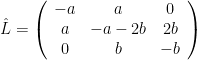$\hat{L} = \left( \begin{array}{ccc} -a & a & 0 \\ a & -a-2b & 2b \\ 0 & b & -b \end{array} \right)$ . This corresponds to "merging" nodes 3 and 4. The non-zero eigenvalues of $\hat{L}$ are the solutions to $4ab + (2a+3b)\lambda + \lambda^2 = 0$ . Since all coefficients are positive, the eigenvalue we are interested in (the smallest in magnitude) is $\lambda = -\frac{(2a + 3b)}{2} + \sqrt{(2a + 3b)^2/4 -4ab}$ . Computing the corresponding eigenvector, we get $v = (1, \frac{a+\lambda}{a}, \left(\frac{a+\lambda }{a}\right)\left(\frac{b+\lambda}{ b}\right)^{-1})$ . Since $\lambda< 0$ and $a < b$ , the maximum of this eigenvector lies indeed at the first coordinate.

Actually, a direct computation shows that the characteristic equation for L itself is $\lambda(b + \lambda)(4ab + (2a+3b)\lambda+ \lambda^2) = 0$ . So, the eigenvalues are the same as for $\hat{L}$ , except that $\lambda = -b$ is an additional eigenvalue. For a non-zero eigenvalue not equal to $-b$ , the corresponding eigenvector is $(1 , \frac{a+\lambda}{a} , \left(\frac{a+\lambda} { a}\right)\left(\frac{b+\lambda} { b}\right)^{-1} , \left(\frac{a+\lambda }{a}\right)\left(\frac{b+\lambda}{b}\right)^{-1})$ . Again, since $\lambda< 0$ , the maximum is attained at coordinate 1. Also, as expected from symmetry, the 3rd and 4th coordinates of the eigenvector are equal.

Comment by Johannes — June 5, 2012 @ 3:16 pm | Reply
- typo: it should be ((a+lam) / a) / ((b+lam) / b) and not ((a+lam) / a)((b+lam) / b)
  
  Edit: Fixed
  
  Comment by Johannes — June 6, 2012 @ 8:01 am | Reply
As I understand your merge, we note that since nodes 3 and 4 will have the same value, we can record that as a single quantity… but really since it is the sum of the heat at nodes 3 and 4 there is twice as much heat flow. So wouldn’t $\hat{L}$ be

$\hat{L} = \left( \begin{array}{ccc} -a & a & 0 \\ a & -a-2b & 2b \\ 0 & 2b & -2b \end{array} \right)$ ?

Comment by Chris Evans — June 6, 2012 @ 1:42 am | Reply
- I got to this formula by considering the Markov process formulation — if we are at 2, we have probability 2*b to go to the “merged node” [3,4] (because we can go to 3 with prob b, or 4 with prob b). However, if we are at [3,4], then we will go to node 2 with probability b only. I think what happens is that the interpretation of the value of eigenvector on this node corresponds to the average of 3 and 4, rather than the sum. But surely your way of merging should work at well. And I’m not really saying that it is useful to merge these nodes at all, I just started the computations that way :)
  
  Comment by Johannes — June 6, 2012 @ 7:35 am | Reply
  - Ah ok I sort of see… in your $\hat{L}$ , the heat coming back in from node 3 is doubled (seen in the (2,3)-entry of $\hat{L}$ )… so it is as though we assume that whatever heat flows in from 3 is matched by the invisible node 4?
    
    In any case $\hat{L}$ seems to work. Indeed, by wolfram alpha, the characteristic polynomial you got for L checks out (and includes that of $\hat{L}$ ):
    
    http://www.wolframalpha.com/input/?i=determinant%28-a-l%2Ca%2C0%2C0%2Ca%2C-a-2b-l%2Cb%2Cb%2C0%2Cb%2C-b-l%2C0%2C0%2Cb%2C0%2C-b-l%29
    
    I then went to compute the eigenvectors using Wolfram Alpha and saw horrific expressions… but then I saw that your eigenvectors were in terms of lambda itself. That makes things more elegant and can perhaps be used to used to prove the conjecture for $G_1$ for arbitrary a<b<c?
    
    Indeed, we seek the null space of $L-\lambda= \left( \begin{array}{cccc} -a-\lambda & a & 0 & 0 \\ a & -a-b-c-\lambda & 0 & 0 \\ 0 & b & -b-\lambda & 0 \\ 0 & c & 0 & -c-\lambda \end{array} \right)$ when $\lambda$ is the second eigenvalue. If we let $v_k$ denote the components of the eigenvector then we can scale so that $v_2=1$ (provided $v_2$ isn’t zero!), whence
    
    $v_1=a/(a+\lambda)$
    
    $v_2=1$
    
    $v_3=b/(b+\lambda)$
    
    $v_4=c/(c+\lambda)$
    
    This is what you had (but rescaled so that $v_2 = 1$ instead of $v_1=1$ in your case). However it isn’t clear to me why $v_1$ and $v_3$ should be the extrema… For one thing, some of the $v_k$ are going to be negative (because we know apriori that the $v_k$ sum to 1 as the second eigenvector is perpendicular to the first) so it must be that $\lambda_2 <-a$ .
    
    If we could show somehow that $-b<\lambda_2<-a$ (and this must be the case since, experimentally, if $v_2=1$ then $v_1$ is negative and $v_3,v_4$ are positive) then we would be done since $v_1$ would be negative and $v_3$ would be the largest of the three positive verticies.
    
    Comment by Chris Evans — June 7, 2012 @ 3:17 am | Reply
[…] is <a href=”https://polymathprojects.org/2012/06/03/polymath-proposal-the-hot-spots-conjecture-for-acute-triangle…” […]

Pingback by Polymath Projects « Euclidean Ramsey Theory — June 6, 2012 @ 9:02 pm | Reply
Here are some few naive observations. None of these provide a roadmap to a proof, but may help build intuition. This is my first post on polymath, so please let me know if more/less detail is required.

First, I’ve taken the liberty of computing, using a finite element method, the desired eigenfunction of the Neumann Laplacian on a couple of acute triangles.

The results are not surprising. I’ve plotted some contour lines as well.

and

The domain is subdivided into a finite number N of smaller triangles. On each, I assumed the eigenfunction can be represented by a linear polynomial. Across interfaces, continuity is enforced.
I used Matlab, and implemented a first order conforming finite element method. In other words, I obtained an approximation from a finite-dimensional subspace consisting of piece-wise linear polynomials. The approximation is found by considering the eigenvalue problem recast in variational form. This strategy reduces the eigenvalue question to that of finding the second eigenfunction of a finite-dimensional matrix, which in turn is done using an iterative method. As N becomes large, my approximations should converge to the true desired eigenfunction. This follows from standard arguments in numerical analysis. I am happy to provide more details if needed.

Additionally, I’ve computed a couple of approximate solutions to the heat equation in acute triangles. The initial condition is chosen to have an interior ‘bump’, and I wanted to see where this bump moved. Again, I’ve plotted the contour lines of the solutions as well, and one can see the bump both smoothing out, and migrating to the sharper corners:

http://people.math.sfu.ca/~nigam/polymath-figures/isoceles.avi
http://people.math.sfu.ca/~nigam/polymath-figures/isoceles2.avi
http://people.math.sfu.ca/~nigam/polymath-figures/scalene.avi

I think in the neighbourhood of the corner with interior angle $\frac{\pi}{\alpha}$ , the asymptotic behaviour of the (nonconstant) eigenfunctions should be of the form 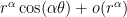$r^\alpha \cos(\alpha \theta) + o(r^{\alpha})$ , where $r$ is the radial distance from the corner.

Next, if one had an unbounded wedge of interior angle $\frac{\pi}{\alpha}$ , the (non-constant) eigenfunctions of the Neumann Laplacian would be given in terms of $P_n(r,\theta) = J_{\alpha, n} (\sqrt(\lambda) r) cos(\alpha n \theta), n=0,1,2....$ . The $J_{\alpha,n}$ are Bessel functions of the first kind. The spectrum for this problem is continuous. When we consider the Neumann problem on a bounded wedge, the spectrum becomes discrete.

This makes me think approximating the second eigenfunction of the Neumann Laplacian in terms of a linear combination of such $P_n(r,\theta)$ could be illuminating.

This idea is not new, and a numerical strategy along these lines for the Dirichlet problem was described by Fox, Henrici and Moler (SIAM J. Numer. Anal., 1967). Betcke and Trefethen have a nice recent paper on an improved variant of this ‘method of particular solutions’ in SIAM Review, v. 47, n. 3, 2005.

Edit: Links to the papers:

http://www.jstor.org/stable/10.2307/2949737

Click to access MPSfinal.pdf

Comment by Nilima Nigam — June 7, 2012 @ 8:20 pm | Reply
- Good stuff. It sounds as though the finite element method is the standard way to approximate the eigenfunctions of the triangle… you mentioned that this led to a finite dimensional linear system/problem for finding the eigenvalue of a matrix. I am curious what the system is (as that may be an entry of attack).
  
  You mention the angle as pi/alpha as opposed to alpha… any reason for this? Also what makes you suspect that $P_n(r,\theta) = J_{\alpha, n} (\sqrt(\lambda) r) cos(\alpha n \theta), n=0,1,2,\ldots$ ? And finally what do you mean by “unbounded/bounded wedge”.
  
  (These may standard concepts in numerical analysis but I am not familiar with them :-/ )
  
  Comment by Chris Evans — June 8, 2012 @ 5:22 pm | Reply
  - Chris, I’ll attempt to answer in reverse order.
    
    – By a wedge I mean the domain $\{(r,\theta)\vert 0\leq r \leq a, 0\leq \theta \leq \frac{\pi}{\alpha}\}$ . An unbounded wedge would have $0\leq r$ . A bounded wedge would have finite a.
    
    – The seperation of variables solution for the Neumann Laplacian on an unbounded wedge is given by $P_n(r,\theta)$ . My thinking is that as one gets close to corners, the behaviour of the true eigenfunction must, in some asymptotic sense, be the same that of $P_n(r,\theta)$ as $r\rightarrow 0^+$ . In other words, if I am very close to a corner of the triangle, the domain appears as if it were an infinite wedge.
    
    – If I were seperating variables on a wedge with angle $\beta$ , solutions would have angular behaviour of the form $\cos(k\frac{\pi \theta}{\beta})$ . I find it easier to set the angle to $\frac{\pi}{\alpha}$ , in which case the angular behaviour is $\cos(k \alpha \theta)$ .
    
    – the finite element matrices I used are quite large, but sparse. It’s a bit unwieldy to post the matrix. But I can attempt to describe it.
    
    The original problem, in variational form, is to find $(u,\lambda)$ such that
    
    $\int_{\Omega} |\nabla u|^2 = \lambda \int_\Omega u^2.$
    
    I am assuming the approximate solution $u_N$ is a linear combination of basis functions $\psi_j$ which are described below. I am attempting to find the first nonzero eigenvalue $\lambda$ and eigenvector $C=(c_1,c_2,...c_N)^T$ such that
    
    $A C = \lambda_N M C.$
    
    The entries of the matrix $A$ would be of form $\int_\Omega \nabla \psi_i \cdot \nabla \psi_j$ . The entries of the matrix $M$ are of form $\int_\Omega \psi_i \psi_j$ .
    
    Suppose for a minute that it were possible to tesselate the acute triangle $\Omega$ by smaller right triangles. The collection of these triangles is called the mesh. Denote such triangle to be $T_h$ . On $T_h$ , we are saying that the desired eigenfunction is well-approximated by a linear polynomial: $a+bx+cy$ . This polynomial is completely specified by its values at the vertices of $T_h$ . Now consider a ‘hat’ function $\psi_i(x,y)$ , which takes on value 1 at the ith vertex of the mesh, 0 on all adjacent vertices, linear in between and zero everywhere else. Clearly a globally piece-wise linear function will be comprised of a linear combination of these hat functions.
    
    Most of the entries of $A$ and $M$ will be zero, since the support of $\psi_i$ does not intersect that of $\psi_j$ unless they are close. The matrices will be symmetric.
    
    Now, we are attempting to do all this on an acute triangle $\Omega$ , so the smaller triangles $T_h$ in our mesh are affine maps of right-angled triangles. So we have to include this map while building the matrices.
    
    To get a ‘feel’ for the sparsity structure of $A$ on an acute triangle using linear FEM, here’s a picture:
    
    Comment by Nilima Nigam — June 8, 2012 @ 7:34 pm | Reply
- Very nice graphics. I might suggest plotting the “line of nodes”, the points where the “heat” is zero, in the first non-trivial eigenfunction. As Terry Tao has discussed, for an equilateral triangle, the first non-trivial eigenvalue for the laplacian with Neumann boundary condition has multiplicity two.
  I’m pretty sure that these Neumann eigenvalues and eigenfunctions also correspond to “pure tones” for a freely vibrating membrane. Wikipedia has (animated) modes for a disk-like drum surface fixed to the rim, which unfortunately is the Dirichlet problem. Speaking non-rigorously, for the Neumann eigenfunctions of a triangle (for non-zero eigenvalue) , the line/curve or “nodal line” should separate the regions of positive heat from those of negative heat. As a visual aid, we could use the “nodal lines” to guide us in finding the hot/cold spot: start from the “nodal line” and do a steepest ascent or steepest descent. Also, I succeeced in downloading the animation isoceles.avi from your website. It was possible using a media player to slow down the replay by 30X, going from 2 to 60 seconds.
  
  Comment by meditationatae — June 14, 2012 @ 5:16 am | Reply
  - There has been some talk of nodal lines in the more recent comments on the second research page. I suspect that the nodal line always straddles the sharpest angle and is bowed out, whence an argument like the one used for the Dirichlet Neumann problem could maybe be put to use. But all of this would require quantitative bounds on the nodal line…
    
    I don’t quite follow the steepest descent proposal… wouldn’t that require lots of knowledge about $u$ itself, in which case we’d know the locations of the max/min already? Or maybe I am missing something?
    
    Comment by Chris Evans — June 14, 2012 @ 8:21 am | Reply
    - I should have been clearer in what I said about the nodal lines.
      I mention these in connection with enhancing the plots for
      eigenfunctions and perhaps for building physical intuition.
      So, I’m assuming we know $u$ already.
      In Nilima Nigam’s figure:
      http://people.math.sfu.ca/~nigam/polymath-figures/isoceles1.jpg ,
      the triangle has a base of length 1 and a height of 2.
      This isosceles triangle has angles of about 28, 76 and 76 degrees,
      so the smallest angle is quite accute. So, certainly here the
      nodal line straddles the sharpest angle and is bowed out (toward
      the base). In an isosceles triangle with angles 80, 50 and 50
      degrees, I really don’t know where the nodal line is for the
      eigenfunction associated to the first non-zero
      eigenvalue … I’ll have to think about it …
      
      Comment by meditationatae — June 14, 2012 @ 10:43 am | Reply
      - After reading Siudeja’s post below, I think the Laugesen and Siudeja paper referred to there implies that an 80, 50, 50 degrees isosceles triangle has its nodal curve for the first eigenfunction along the bisector of the 80-degree angle. (See Figure 1 of the Laugesen and Siudeja paper, for example)
        
        Comment by meditationatae — June 14, 2012 @ 11:33 am | Reply
        
        It’s easy enough for me to generate some figures showing the nodal line for a few triangles.
        As for your steepest descent comment:
        
        do you mean we should plot the nodal line in the same fixed triangle as time increases (in the heat equation), and then look at the direction of steepest descent? This is relatively easy to do.
        
        or do you mean we should plot the nodal line for triangles with angles which are close, and somehow study the nodal lines in there? This I don’t readily see how to do, since the domain (and hence the location of the nodal lines) will change from triangle to triangle.
        
        Let me know if this is still of interest, and I can throw up some graphics.
        
        Comment by Nilima Nigam — June 14, 2012 @ 2:47 pm | Reply
        
        I’ll explain why lines of steepest descent interest me. They are evevrywhere tangent to the gradient of $u$ , the lowest non-trivial eigenfunction of the Neumann Laplacian. For your height 2 , base 1 isosceles triangle, it seems the “cold spot” has $u$ about -0.09 , at the pointy vertex. Maybe we already know that the two other vertices at the base are the only two “hot spots” with $u$ being about +0.03 there, and maybe +0.025 on the base, half-way between the two “hot spot” vertices. Say we do a mirror image of the 3d graph of $u$ about the base, thus extending $u$ ; could it be that the extended $u$ has a saddle point at x=0, y=0 ? It seems that to the left of the axis of symmetry of the height 2, base 1 triangle, the steepest ascent curves should slope downwards and to the left, and to the right of the axis of symmetry, the steepest ascent curves starting at the pointy vertex should slope downwards and to the right.
        For nodal lines, I meant for the eigenfunctions. They show where $u$ is average-valued. For the isosceles case, we already know where they lie, by the of Laugesen and Siudeja.
        
        Comment by meditationatae — June 14, 2012 @ 3:58 pm | Reply
Is the case of an isosceles triangle still open?

I was thinking of the following. Say the triangle has vertices $(a,0)$ , $(-a,0)$ and $(0,h)$ . If $u(x,y)$ is the second eigenfunction, then also is $u(-x,y)$ and their sum $v(x,y)=u(x,y)+u(-x,y)$ . The function v is even in x, so it is also a Neumann eigenvalue of the right triangle with vertices $(0,0)$ , $(0,h)$ and $(a,0)$ . According to the description of the problem the case of the right triangle has already been worked out, so this would reduce to that case unless v is identically zero.

If v is identically zero, it means that the second eigenfunction u was odd in x. In particular $u(0,y)=0$ for all y. The function u would be the first eigenfunction on the same right triangle as above but now with Dirichlet boundary condition on x=0 and Neumann in the other two edges. This function cannot change sign (otherwise |v| has less energy). I would expect its maximum to take place at (a,0) but I don’t know how to prove it (maybe some rearrangement along lines?).

Comment by Luis S — June 7, 2012 @ 10:05 pm | Reply
- As far as I know, the case for a general isoceles triangle is open, but don’t quote me on that :) Of course some cases like obtuse-isoceles are solved.
  
  I believe the obtuse-isoceles triangle has an anti-symmetric secong eigenfunction and the acute-isoceles triangle has a symmetric second eigenfunction (as this follows the hueristic that the hot spots are in the sharpest corners.)
  
  When you reduce to the case of the right triangle in your first paragraph, how do you know that it is still the second eigenfunction(as opposed to some other eigen function)?
  
  Comment by Anonymous — June 8, 2012 @ 9:35 pm | Reply
  - Because any other eigenfunction of the right triangle would produce a corresponding even eigenfunction of the isosceles triangle.
    
    Of course I can’t rule out the second eigenfunction of the isosceles to be odd.
    
    Comment by Luis S — June 10, 2012 @ 1:37 am | Reply
    - According to Proposition 2.3 of the Banuelos-Burdzy paper, the second eigenfunction of a symmetric domain cannot be odd if the ratio between the diameter and the width is at least $2 j_0/\pi \approx 1.53$ , where $j_0$ is the first non-trivial zero of the Bessel function J_0. So this handles isosceles triangles which are sufficiently pointy, at least…
      
      Comment by Terence Tao — June 10, 2012 @ 1:53 am | Reply
      - The isoceles right-angled triangle has diameter of twice the width, so I’m not sure the ratio isn’t at least 1.53 for all acute isoceles triangles.
        
        Comment by Lior Silberman — June 11, 2012 @ 11:46 pm | Reply
        
        Should have been more careful: only the width perpendicular to the axis of symmetry counts.
        
        Comment by Lior Silberman — June 11, 2012 @ 11:47 pm | Reply
        
        Unfortunately so :-). Note that for the equilateral triangle there do exist odd second eigenfunctions (the second eigenspace is two-dimensional, and for each axis of symmetry there is one eigenfunction which is odd and one which is even with respect to that axis), so this method has to break down before that point. Using the Banuelos-Burdzy bound, one can handle all isosceles triangles whose apex has angle less than 38 degrees.
        
        Comment by Terence Tao — June 12, 2012 @ 3:05 am | Reply
- It seems that this argument almost resolves the hot spots conjecture in the case of a narrow isosceles triangle (in which Banuelos-Burdzy excludes the possibility of an odd eigenfunction), except for the following issue: an even eigenfunction on the isosceles triangle is indeed also a Neumann eigenfunction on one of the two right-angled halves of that triangle, and hence by the hot spots conjecture for right-angled triangles (which follows, among other things, from this paper of Atar-Burdzy which covers the lip domain case), the extrema can only occur on the boundary of the right triangles. Unfortunately this also includes the axis of symmetry of the original triangle as well as the boundary of that triangle; if we can exclude an extremum occuring in the interior of this axis of symmetry then we are done. I think there are some extra monotonicity properties known for eigenfunctions of right triangles that can be extracted from the Atar-Burdzy paper which may be useful in this regard; I’ll go have a look.
  
  Comment by Terence Tao — June 11, 2012 @ 6:16 pm | Reply
  - Aha! It appears that in Theorem 3.3 of the Banuelos-Burdzy paper it is shown that in a right-angled triangle ABC with right angle at B, if the second eigenfunction is simple, then (up to sign) it is non-decreasing in the AB and BC directions, which among other things shows that it cannot have an extremum in the interior of AB or BC (without being constant on those arcs, which by unique continuation would make the entire eigenfunction trivial). So, putting everything together, it seems that this implies that the hot spots conjecture is true for thin isosceles triangles, and more generally for isosceles triangles in which the second eigenfunction has multiplicity one and is even. I’ve written up the details on the wiki: http://michaelnielsen.org/polymath1/index.php?title=The_hot_spots_conjecture#Isosceles_triangles
    
    Comment by Terence Tao — June 11, 2012 @ 6:31 pm | Reply
I wanted to suggest another approach to the problem using the connection between the Laplacian and Brownian motion.

Suppose I start off a Brownian motion at time 0 at some point $x$ in the triangle, and the Brownian motion reflects off the sides of the triangles. At time $t$ the probability density for the Brownian motion to be at location $y$ is given by the solution $v(t,y)$ of the heat equation with $v(0,y)=\delta(x-y)$ and Neumann boundary conditions. So if I can show that the Brownian motion is eventually more likely to be in a corner (per unit area) than anywhere else, that will gives us the result.

Here’s a way to approach it: Suppose I fix $x$ . I ask how many ways are there for Brownian motion to get from $x$ to $y$ in time $t$ . For $t$ large, If $y$ is in a corner I might imagine that there are more ways of Brownian motion to get to $y$ than otherwise, because the Brownian motion has all the ways it would in free space, but also a ton of new ways that involve bouncing off the walls. Perhaps you can using some argument showing that there are more paths into some corners than anywhere else in the triangle. (Perhaps, using the Strong Markov Property and Coupling?)

Comment by paultupper — June 8, 2012 @ 5:36 pm | Reply
- Sorry, I just realized that Chris had already proposed this approach in
  
  Click to access Polymath.pdf
  
  and reference the following paper where they do something similar.
  http://en.scientificcommons.org/42822716
  
  Comment by paultupper — June 8, 2012 @ 7:16 pm | Reply
If we could find an heat distribution on a right triangle such that the hot spot is never on the vertices or the hypotenuse or the short side then could we combine two such heat distributions symmetrically in an isosceles acute triangle and get an isosceles acute triangle such that the hot spots are always on the interior?

Does such a distribution exist? Is it among the known possibilities?

Comment by Kristal Cantwell — June 8, 2012 @ 8:46 pm | Reply
- An issue is that if you reflect a right triangle and its eigenfunction the eigenfunction you get for the larger triangle might not be the *second* eigenfunction.
  
  Comment by Anonymous — June 8, 2012 @ 9:40 pm | Reply
- Theorem 3.3 of Banuelos-Burdzy shows that in a right angled triangle, the hot spots of the second eigenfunctions are only at the two acute vertices, so this potential counterexample is ruled out.
  
  Comment by Terence Tao — June 12, 2012 @ 3:06 am | Reply
Thanks for the detailed details. It seems the problem you want to solve is $c^TAc = \lambda_N c^tMc$ ? But solving $Ac=\lambda_N Mc$ suffices (Maybe it is a necessary condition too?)

But in any case it seems that the finite element method doesn’t lead to a problem of “find the eigenvector of this matrix” so much as “solve this linear system”. So in that sense it seems fundamentally different from the approach using graphs $G_n$ that I proposed (though I still suspect that the graphs $G_n$ correspond to some finite element method?)

Looking at the structure of $u_N$ , it is clear that its maximum will occur at one of the verticies of the mesh… that is, the hotspots conjecture for the finite elements would be the claim that “For each N, the vector c is such that the extrema of c correspond to verticies of the mesh which are on the boundary of the big triangle (and most likely should in fact be at the sharpest corners of the big triangle)”. So maybe that can be shown somehow

As to the eigenfunction near the corner looking like the eigenfunction of the wedge, it certainly sounds plausible but I am not sure what the heuristic argument would be. If I start a point mass of heat in the corner and let heat flow, then for a *short* time t, I don’t expect the heat flow to differ from the heat flow in a wedge (not enough time has elapsed for much heat to have reflected off the third side of the triangle). But for *long* time (which is where the second eigenfunction comes into play) it seems like the third side of the triangle should matter. But what you are saying does still “feel” right in that I would be surprised if it weren’t the case.

Speaking of wedges, it must be the case that the heat flow on the infinite wedge of angle $\alpha = \frac{2\pi}{N}$ can be obtained as follows: Divide, centered at the origin, your space into wedges $j*\frac{2\pi}{N} < \theta < (j+1)*\frac{2\pi}{N}$ . Then look at the unreflected heat flow on $R^2$ and then "fold up" (as in origami) $R^2$ into a single wedge adding up the values of heat. In the case of an equilateral triangle it must be possible to tile $R^2$ with the triangle, look at the unreflected heat flow, and then "fold it up" as well. Perhaps some trick involving folding can be used for a general triangle?

Comment by Chris Evans — June 9, 2012 @ 4:42 am | Reply
- Chris, you’re right about the transposes: the eigensystem to solve is
  
  $AC^T =\lambda_N MC^T.$
  
  I think your rephrasing of the conjecture in this setting is promising. The acuteness of the angle would need to be built into the interpretation somehow, since the entries of the matrices involved will be affected by the affine maps from the reference right triangles to the tesselating ones. I believe this is key.
  
  A decent way to start may be to begin with an isoceles triangle, divide it into 6 smaller right triangles, and explicitly write down the resulting matrices. The approximation $u_6$ will unfortunately be a lousy approximation to the true eigenfunction,but the exercise may still be illuminating.
  
  I think that because the sharper corner will be further from the third side, it will take longer for a bump to diffuse from there to the third side. It will dissipate faster due to the exponential decay in time of the second eigenfunction. This was the heuristic I was using.
  
  Comment by Nilima Nigam — June 9, 2012 @ 5:03 am | Reply
[…] “Hot spots conjecture” proposal has taken off, with 42 comments as of this time of writing. As such, it is time to take the […]

Pingback by Polymath7 discussion thread « The polymath blog — June 9, 2012 @ 5:51 am | Reply
- As you can see, I’ve just officially designated this project as the Polymath7 project, and created a discussion page (for all meta-mathematical discussion of the project at https://polymathprojects.org/2012/06/09/polymath7-discussion-thread/ ) and a wiki page (at http://michaelnielsen.org/polymath1/index.php?title=The_hot_spots_conjecture ) for holding all the progress to date. I’m also going through the comments to clean up the LaTeX (see https://polymathprojects.org/how-to-use-latex-in-comments/ ).
  
  One slightly more mathematical question: what is the reference for the fact that the hot spots conjecture is resolved in the right-angled case? Does the Banuelos-Burdzy result cover this case?
  
  Also, in addition to the perturbed right-angled triangle case proposed earlier, another case that might be easier than the general case is that of an almost degenerate triangle, in which the three vertices are nearly collinear. It may be that in that case one can use perturbative techniques to get asymptotics for the second eigenfunction that can solve the conjecture for sufficiently degenerate triangles (and, if one is optimistic, maybe one could then use a continuity argument to push to the general case)…
  
  Comment by Terence Tao — June 9, 2012 @ 5:57 am | Reply
  - The article:
    
    The “Hot Spots” Conjecture for Domains with Two Axes of Symmetry
    David Jerison and Nikolai Nadirashvili
    Journal of the American Mathematical Society
    Vol. 13, No. 4 (Oct., 2000), pp. 741-772
    
    which is available at http://www.math.purdue.edu/~banuelos/Papers/hotarticle.pdf
    
    seems to imply that if a convex region as symmetries in the x and y axes then the conjecture will hold.
    
    Since four copies of a right triangle can be combined to from such a region then they should satisfy the cojecture. Also two copies of a isoceles triangle could be combined to form such a region so they should also satisfy the conjecture.
    
    Comment by Kristal Cantwell — June 9, 2012 @ 5:04 pm | Reply
    - What worries me is that if you create a larger domain by reflection (and reflecting the eigenfunction), there is no guarantee that the resulting eigenfunction is still the second eigenfunction of the larger domain.
      
      A (possibly incorrect but plausible) heuristic is that larger domains have a smaller (i.e. closer to zero) second eigenvalue (because in a larger domain it takes longer for the heat to reach equilibrium maybe?). If that is the case then it would be legal to make arguments on “folding in” a triangle (e.g. replacing an isosceles triangle with the one you get by folding it in half) but illegal to make arguments on “unfolding” a triangle (e.g. replacing a right triangle with the isosceles triangle it folds out to).
      
      At least in the case of an obtuse isosceles triangle with angles $\alpha=\alpha < \frac{\pi}{2} < \gamma$ , the second eigenfunction seems to be anti-symmetric with its extrema at the corners of angle $\alpha$ . If this is "folded in" you get the function which is identically zero. On the other hand, if you start with the right triangle with angles $\alpha,\frac{\pi}{2}, \frac{\gamma}{2}$ and consider its second eigenfunction, when you "unfold it" to the obtuse isosceles triangle from before, while it is still an eigenfunction of the larger triangle, it is not the second eigenfunction (which was antisymmetric).
      
      If it is true that "folding in" is "legal", it may be possible to fold in an isosceles triangle as Luis S. suggested above to furnish a proof.
      
      Comment by Chris Evans — June 9, 2012 @ 6:59 pm | Reply
      - Together with Richard Laugesen (see “Minimizing Neumann fundamental tones of triangles: an optimal Poincaré inequality”. J. Differential Equations, 249(1):118-135, 2010) I showed that second eigenfunction for isosceles triangles is symmetric for “tall” isosceles triangles (angle below pi/3) and antisymmetric for “wide” isosceles triangles (angle above pi/3). The transition is at equilateral, with both cases having the same eigenvalue.
        
        This also means that a half of a “tall” isosceles triangle has the same second eigenfunction as the whole isosceles triangle. In general for Neumann boundary conditions there is no domain monotonicity. One can take a rectangle where the second eigenfunction is based on the longer side and put another one inside of it, along diagonal, that has longer long side. This will give a much smaller domain contained in a larger one, but with smaller eigenvalue.
        
        Comment by Bartlomiej Siudeja — June 12, 2012 @ 5:32 pm | Reply
        
        Very nice! Combining this with Luis’s argument and Banuelos-Burdzy’s monotonicity, it now appears that we have the hot spots conjecture for all subequilateral isosceles triangles. It seems like the superequilateral isosceles case is the one to focus on next… now we have odd eigenfunctions and so we have to somehow understand mixed Dirichlet-Neumann lowest eigenfunctions on right-angled triangles…
        
        Comment by Terence Tao — June 12, 2012 @ 7:09 pm | Reply
  - For this, perhaps start with a thin wedge $\Omega:= \{(r,\theta)\vert 0< r< R, 0< \theta< \epsilon\} <$ The second Neumann eigenfunction can be written down on this explicitly. Now consider a process of deforming the domain whereby the curvilinear piece $r=R$ of the boundary $\partial \Omega$ is slowly flatted to a line segment.
    
    Comment by Nilima Nigam — June 9, 2012 @ 7:29 pm | Reply
    - That’s a good idea; I’ll try computing the details. A related thought I had was to start with a thin isosceles triangle (say with vertices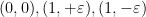 $(0,0), (1,+\varepsilon), (1, -\varepsilon)$ ), take the second eigenfunction $u_\varepsilon$ (normalized in $L^2$ , say), rescale it to a fixed triangle (say with vertices 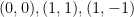$(0,0), (1,1), (1,-1)$ by considering the rescaled function $\varepsilon^{1/2} u_\varepsilon(x, \varepsilon y)$ , and investigate what happens in the limit $\varepsilon \to 0$ (I believe there is enough compactness to extract a useful limit, but haven’t checked this yet). My guess is that the limit should obey some exactly solvable ODE, but I haven’t worked out the details yet; I should probably do the sector case first to build some intuition.
      
      Comment by Terence Tao — June 9, 2012 @ 8:33 pm | Reply
      - Well, the sector $\{ (r \cos \theta, r \sin \theta): 0 \leq r \leq R; 0 \leq \theta \leq \alpha \}$ at least was easy to work out. By separation of variables, one can use an eigenbasis of the form $u(r,\theta) = u(r) \cos \frac{\pi k \theta}{\alpha}$ for $k=0,1,2,\ldots$ . For any non-zero k, the smallest eigenvalue of that angular wave number is the minimiser of the Rayleigh quotient 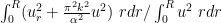$\int_0^R (u_r^2 + \frac{\pi^2 k^2}{\alpha^2} u^2)\ r dr / \int_0^R u^2\ r dr$ ; the $k=0$ case is similar but with the additional constraint $\int_0^R u\ r dr = 0$ . This already reveals that the second eigenvalue will occur only at either k=0 or k=1, and for $\alpha$ small enough it can only occur at $k=0$ (because the $k=1$ least eigenvalue blows up like $1/\alpha^2$ as $\alpha \to 0$ , while the $k=0$ eigenvalue is constant).
        
        Once $\alpha$ is small enough that we are in the k=0 regime (i.e. the second eigenfunction is radial), the role of $\alpha$ is no longer relevant, and the eigenfunction equation becomes the Bessel equation 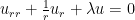$u_{rr} + \frac{1}{r} u_r + \lambda u = 0$ , which has solutions $J_0(\sqrt{\lambda} r)$ and $Y_0(\sqrt{\lambda} r)$ . The $Y_0$ solution is too singular at the origin to actually be in the domain of the Neumann Laplacian, so the eigenfunctions are just $J_0(\sqrt{\lambda} r)$ , with $\sqrt{\lambda} R$ being a zero of $J'_0$ . The second eigenfunction then occurs when $\sqrt{\lambda} R$ is the first non-trivial zero of $J'_0$ ( $3.8317\ldots$ , according to Wolfram alpha). This is a function with a maximum at the origin and a minimum at the circular arc, consistent with the hot spots conjecture.
        
        Now I’ll try to see what happens for a thin isosceles triangle…
        
        Comment by Terence Tao — June 9, 2012 @ 9:18 pm | Reply
      - I think the case of a thin isosceles triangle $T_\varepsilon$ with vertices $(0,0),(1,+\varepsilon), (1,-\varepsilon)$ is also going to be OK. Let $u_\varepsilon$ be a $L^2$ normalised second eigenfunction on $T_\varepsilon$ with eigenvalue $\lambda_\varepsilon$ , thus $\int_{T_\varepsilon} u_\varepsilon^2 = 1$ , and by integration by parts $\int_{T_\varepsilon} |\nabla u_\varepsilon|^2 = \lambda_\varepsilon$ and $\int_{T_\varepsilon} |\nabla^2 u_\varepsilon|^2 = \lambda_\varepsilon^2$ . Ideally I would like to continue integrating by parts but I am having a bit of trouble dealing with the boundary terms; still the theory of regularity of Neumann eigenfunctions on a domain as nice as a triangle is presumably very well developed, so let me assume that we can get higher regularity bounds also.
        
        Using a Poincare inequality, I think one can show that $\lambda_\varepsilon$ is bounded above uniformly in the limit $\varepsilon \to 0$ , and by perturbing the Bessel function example from the sector case I think one can also get a bound from below. So (after passing to a subsequence if necessary) we can assume that $\lambda_\varepsilon$ converges to a limit $\lambda$ as $\varepsilon \to 0$ .
        
        Now we look at the rescaled functions $v_\varepsilon(x,y) := \varepsilon^{1/2} u_\varepsilon(x,\varepsilon y)$ on the triangle $T_1$ . These functions have unit norm $L^2$ , and obey the $H^1$ bounds
        
        $\int_{T_1} |\partial_x v_\varepsilon|^2 + \varepsilon^{-2} |\partial_y v_\varepsilon|^2 = O(1)$
        
        and the $H^2$ bounds
        
        $\int_{T_1} |\partial_{xx} v_\varepsilon|^2 + \varepsilon^{-2} |\partial_{xy} v_\varepsilon|^2 + \varepsilon^{-4} |\partial_y v_\varepsilon|^2 = O(1)$ .
        
        This gives enough compactness to let $v_\varepsilon$ converge strongly in H^1 and weakly in H^2 (again after passing to a subsequence) to some limit $v$ , which will be constant in the y direction, thus $v(x,y) = v(x)$ .
        
        Now, the functions $v_\varepsilon$ obey the PDE
        
        $\partial_{xx} v_\varepsilon + \varepsilon^{-2} \partial_{yy} v_\varepsilon + \lambda_\varepsilon v_\varepsilon = 0$
        
        and the boundary conditions
        
        $\partial_y v_\varepsilon = \pm \varepsilon^2 \partial_x v_\varepsilon$
        
        when $y = \pm x$ . We rewrite the PDE as
        
        $\partial_{yy} v_\varepsilon = \varepsilon^2 (-\partial_{xx} v_\varepsilon - \lambda_\varepsilon v_\varepsilon).$
        
        The RHS is $\varepsilon^2 (- v''(x) - \lambda v(x))$ plus errors which are $o(\varepsilon^2)$ in some suitable function norm. Integrating this in y (from -x to x) and comparing with the boundary condition, we get that
        
        $2 \varepsilon^2 v'(x) + o(\varepsilon^2) = 2x \varepsilon^2 ( -v''(x) - \lambda v(x) ) + o(\varepsilon^2)$
        
        and thus on taking limits we see that v obeys the Bessel equation
        
        $v'' + v'/x + \lambda v = 0$ .
        
        The same sort of analysis as in the sector case then tells us that v has to be (a constant multiple of) $J_0(\sqrt{\lambda} x)$ with $\sqrt{\lambda}$ being the first root of J’_0, so it has a non-degenerate maximum at x=0 and non-degenerate minimum at x=1. Hopefully, there is enough uniform regularity on the $v_\varepsilon$ to then conclude that $\partial_{xx} v_\varepsilon$ is bounded away from zero near x=0 and x=1 for $\varepsilon$ small enough, which (in conjunction with the convergence properties of $v_\varepsilon$ to $v$ , and the Neumann boundary conditions) should ensure that $v_\varepsilon$ still has a non-degenerate maximum at x=0 and a non-degenerate minimum at x=1. This would resolve the hot spots conjecture for all sufficiently degenerate isosceles triangles.
        
        Comment by Terence Tao — June 9, 2012 @ 10:09 pm | Reply
        
        This is great!
        
        I think I have some idea on how to obtain the lower bound on the eigenvalue through an analytic perturbation argument from the sector. I’ve put these on the wiki under the ‘thin sector’ section.
        
        Comment by Nilima Nigam — June 10, 2012 @ 2:45 am | Reply
  - Actually, this could be used to good realistic effcet. Sediment will tend to deposit in concavities and wind will tend to clean and abrade convexities giving them different colors. This is much the way that vegetation and sand distribution can be affected by slope. Also, if this could be applied to heightfields or masks, you could use this to flatten out the bottoms of concavities and convexities and possibly to give more of a streaky and abraded or bare rock texture to convexities. I may have to get one of those evil Windows machines just for your app.
    
    Comment by Colleen — August 5, 2012 @ 1:44 am | Reply
[…] 7 is officially underway. It is here. It has a wiki here. There is a discussion page here. Like this:LikeBe the first to like this […]

Pingback by Polymath 7 « Euclidean Ramsey Theory — June 9, 2012 @ 5:22 pm | Reply
Here is a probabilistic argument that seems to mostly prove the conjecture for the graph $G_1$ :

http://www.math.missouri.edu/~evanslc/Polymath/TwoWalkers

Of course, as the graph Laplacian for $G_1$ is just a 4×4 matrix, this is probably unnecessarily complicated.

Comment by Chris Evans — June 9, 2012 @ 7:21 pm | Reply
- Chris, Thanks for this note. It’s very clear. Do you think it’s possible to do a similar coupling if instead of your $G_n$ for $n>1$ you use a different graph that approximates the triangle? I was thinking of just taking a fine rectangular grid and just trimming everything that falls outside the triangle.
  
  Comment by paultupper — June 10, 2012 @ 3:57 pm | Reply
  - It may be possible… it would all come down to finding the correct “action charts” (coupling). I did play around with a few different graphs a while back to no avail, but it may be that I didn’t come across the correct one. It may also help to take advantage of relations between $a,b,c$ besides just the fact that $a<b<c$ . For example, we know that $a<b+c,\ b<a+c$ , and $c<a+b$ .
    
    As this idea is ultimately derived from that in the Banuelos and Burdzy paper, I was hoping that at least it might work in the case where the triangle is obtuse (which would impose an additional relation between $a,b,$ and $c$ … but I haven't managed to make it work there.
    
    Ultimately, however, what the argument in Banuelos and Burdzy paper showed is that obtuse triangles are "monotonicity preserving" which is a stronger property than just having the extrema of the second eigenfunction in corners. If the acute triangles are not monotonicity preserving then such a coupling argument may not be useful.
    
    So this does lead to another question: Are acute triangles monotonicity preserving in any sense? Computer simulation might show this not to be the case. Also, as a side question, is there any way to characterize monotonicity preserving in terms of the eigenfunctions of the Laplacian?
    
    Comment by Chris Evans — June 10, 2012 @ 6:18 pm | Reply
It occurs to me that there is a chance of establishing the conjecture for acute triangles by rigorous numerics. Once one can deal the boundary case of nearly degenerate acute triangles (in which one angle is very small), the remaining configuration space is compact. If we can verify the conjecture for a sufficiently dense mesh of possible angles $(\alpha,\beta,\gamma)$ of acute triangles, and also get some stability for each triangle in the mesh (in particular, by showing that all other stationary points of the eigenfunction are well away from the maximum and minimum, and that the second derivatives have some lower bound at the critical points) then one may be able to cover all possible cases. This wouldn’t be a very elegant way to solve the problem, but it would at least be a solution.

Comment by Terence Tao — June 9, 2012 @ 10:59 pm | Reply
- Just to clarify: by dense mesh of possible angles, do you mean a dense subset of $\mathbb{R}^3$ , with each point corresponding to a triangle?
  
  The challenge I foresee with a purely numerical attack with the usual tools is the following. There will be three levels of approximation. The first will be due to approximating the eigenfunctions by functions in a finite-dimensional function space (it may, or may not, be a subset of $H^1$ depending on the choice of method). The second will be due to computing the discrete eigenfunctions and eigenvalues by an iterative process. The third will be sampling enough acute triangles. We won’t be getting the true eigenvalues or eigenfunctions except in very special circumstances.
  
  I think that since the standard numerical error estimates for eigen-pair calculations rely on the domain shape, it would be challenging to get approximations of equal quality on the dense mesh you describe.
  
  Comment by Nilima Nigam — June 10, 2012 @ 4:13 am | Reply
  - Well, the problem is invariant under scaling, so we don’t need to specify the sides, only the angles. As the angles add up to pi, there are only two degrees of freedom, so the mesh will be in a compact subset of ${\bf R}^2$ rather than ${\bf R}^3$ .
    
    It is true that we can only hope to get approximate eigenfunctions, but this may be good enough using the Rayleigh quotient formalism to get good bounds on eigenfunctions of nearby triangles (assuming that one has lower bounds on the spectral gap between the second eigenvalue and the third eigenvalue of the triangle in the mesh). The one catch is that one needs rather high regularity bounds in order to prevent the maximum or minimum from migrating off of an edge or corner into the interior; something like uniform bounds on the second derivative may be needed.
    
    I’m starting to look at the literature on stability of the second eigenfunctions of the Neumann problem. I found a paper of Carmona and Zheng at http://www.sciencedirect.com/science/article/pii/S0022123684710858 which looks promising, but haven’t digested it yet. But there is a paper of Banuelos and Pang at http://www.emis.de/journals/EJDE/2008/145/banuelos.pdf which shows (among other things) that if one perturbs a triangle by a small amount, then the second eigenvalue only moves by a small amount, and (in the case of simple spectrum) the second eigenfunctions of the perturbation converge uniformly to second eigenfunctions of the original triangle in the limit.
    
    Comment by Terence Tao — June 10, 2012 @ 3:02 pm | Reply
    - In terms of the regularity of eigenfunctions, I think the stability of the almost-degenerate case will be most useful to start with. There are some results about the regularity of eigenfunctions in polygons, depending on the interior angles. The larger the angle, the worse the regularity – but for triangles, we have no re-entrant corners, so I think we will be able to find good bounds on weak second derivatives.
      
      Here are another couple of references which may be of interest. I unfortunately don’t have access to the books until Tuesday.
      
      – Grisvard’s book on Elliptic PDE in Nonsmooth Domains. I have a recollection that Chapter 2 considers the regularity of eigenfunctions in terms of interior angles.
      
      – Babuska and Osborn’s lovely chapter in the Handbook of Numerical Analysis, and in their quest for error estimates for the approximations, provide some estimates on higher derivatives of the eigenfunctions themselves:
      http://www.sciencedirect.com/science/article/pii/S1570865905800420
      
      – Rodriguez and Hernandez consider the case of the eigenvalues of the shifted Laplacian $-\Delta u + u$ and consider a variational approach. Estimate (2.10) in their paper bounds the $H^{1+\alpha}$ norm of the eigenfunction, where $\alpha$ depends on the interior angles of the polygon under consideration. For the triangle, $\alpha =1$
      
      Click to access S0025-5718-02-01467-9.pdf
      
      Comment by Nilima Nigam — June 10, 2012 @ 3:49 pm | Reply
A trivial remark: the second eigenfunction on any domain cannot have both a strict local maximum and a strict local minimum in the interior of the domain. This is because one could shave a little bit off of both the local maximum and the local minimum to reduce the Rayleigh quotient while still staying mean zero, contradicting the fact that the second eigenfunction must minimise the Rayleigh quotient on mean zero functions.

Comment by Terence Tao — June 10, 2012 @ 12:55 am | Reply
- I don’t quite see it. If you shave the max and min certainly the integral of grad square goes down, but also does the L^2 norm in the denominator of the Rayleigh quotient.
  
  Comment by Luis S — June 10, 2012 @ 2:08 am | Reply
  - Oops, you’re right; I had thought that the decrease of the L^2 norm was lower order, but on revisiting the computation I see that they both decrease proportionally, so what I said was nonsense.
    
    [EDIT: in fact, there is a construction of Bass and Burdzy at http://projecteuclid.org/DPubS?service=UI&version=1.0&verb=Display&handle=euclid.dmj/1092403814 which gives a counterexample to the hot spots conjecture (for a domain with holes) in which both the maximum and minimum are attained in the interior.]
    
    Comment by Terence Tao — June 10, 2012 @ 3:13 am | Reply
    - I think I understand the idea in (22), and finding a perturbation that makes the Rayleigh quotient strictly decrease is the difficulty. For the one-dimenional domain [0, 1], I’ve calculated that u(x) = cos(Pi x) is the first eigenfunction for the Laplacian on [0, 1] with a Neumann boundary condition. If a mean zero
      u’ on [0, 1] has a strict local max. in the open interval (0, 1), is it easy to perturb u’ while keeping the mean at zero and decreasing the Rayleigh quotient? (technically, the Rayleigh quotient of the negative of the Laplacian, so that the first non-trivial eigenvalue of the negative Laplacian on [0, 1] with Neumann boundary condition is pi^2 ).
      
      Comment by meditationatae — June 12, 2012 @ 8:31 pm | Reply
To record another idea: the Schwartz-Christoffel map from the upper half plane to the interior of a triangle with angles $\pi a,\pi b$ , and $\pi(1-a-b)$ is given by

$z=f(\zeta)=\int^\zeta \frac{dw}{(w-1)^{1-a} (w+1)^{1-b}}$ .
(I got this from http://en.wikipedia.org/wiki/Schwarz%E2%80%93Christoffel_mapping). The mapping is bijective and biholomorphic. The question about the second eigenfunction of the Neumann Laplacian on the triangle will be converted to a question about the second eigenfunction of a different operator (one which explicitly includes the angles in its symbol).

What might one gain from this approach? One moves to working on a fixed domain (the upper half plane) with a variable operator, instead of all acute angles with a fixed operator (the Laplacian). I have not yet worked out what the variable operator looks like, but perhaps someone already knows a good reference? Zeev Nehari’s book may have the desired identity.

Comment by Nilima Nigam — June 10, 2012 @ 4:24 am | Reply
- this approach is harder than necessary. The map $\left( \begin{array}{cc} a_1 & a_2 \\ 0 & b_2 \end{array} \right)$ takes me from the right triangle $(0,0), (1,0), (0,1)$ to the acute triangle $(0,0), (a_1,0), (a_2,b_2)$ . This map is affine, so calculating pullbacks is not hard. One immediately sees the importance of the nearly-degenerate case, since in this instance the Jacobian of transformation is large.
  
  The Ritz quotient on the acute triangle can be computed in terms of functions on the right triangle, with the angles of the acute triangle appearing explicitly. Pull-backs of minimizers of the (appropriate) Ritz quotient on the acute triangle will be minimizers of the appropriate functional expressed on the right triangle.
  
  I’ll type this up with details for the wiki.
  
  Comment by Nilima Nigam — June 10, 2012 @ 10:01 pm | Reply
  - One advantage of the Schwartz-Christoffel approach (as opposed to the affine approach) is that it preserves the Neumann boundary condition, which is useful if one wants to perform reflection techniques. Also the Laplacian just gets multiplied by a conformal factor, transforming the original eigenfunction equation $-\Delta u= \lambda u$ into a weighted eigenfunction equation $-\Delta u = \lambda \Omega u$ for some fixed weight function $\Omega$ . The downside is of course that this weight is somewhat messy…
    
    Comment by Terence Tao — June 12, 2012 @ 2:48 am | Reply
    - Good point!
      
      My motivation for doing this calculation is to attempt what you suggested in Thread 21 above. In essence, getting a numerical approximation via the Schwartz mapping will be slower than using a finite element strategy on the mapped triangle. So we decided to come up with an efficient yet robust approximation method, which could be used to probe parameter space fast.
      
      Joe Coyle and I did the calculations for the affine-mapped triangle, and it doesn’t look too bad. The Ritz quotient is modified, but by a matrix which has constant entries; the eigenvalue problem for the Laplacian is recast into one for an elliptic operator but with constant coefficients. We’ve written down two formulations of the problem on the wiki.
      
      Such calculations are frequently seen in the finite element literature (we used the book by Peter Monk on Finite Element Methods for Maxwell’s Equations).
      
      I’m a bit worried about garbling the calculation on this blog, and have typed it up on the wiki:
      
      http://michaelnielsen.org/polymath1/index.php?title=The_hot_spots_conjecture#Computational_strategies
      
      We have some preliminary code running. Once we’re confident it is working, we’d be happy to test regions of parameter space you think are of interest.
      
      Comment by Nilima Nigam — June 12, 2012 @ 3:51 am | Reply
      - To record one of our reformulations here: let the acute triangle have corners $(0,0), (a_1,0), (a_2,b_2)$ and the reference triangle have corners $(0,0), (1,0), (0,1)$ .
        
        Let $B:= \left(\begin{array}{cc} a_1 & a_2\\ 0 & b_2\end{array} \right)$ . This is the matrix corresponding to the map which takes the reference triangle to the acute one.
        
        The Neumann problem for the non-constant eigenfunctions is to find
        $(\hat{u}, \lambda)$ so that
        
        $\displaystyle -\nabla \cdot (M \nabla \hat{u}) = \lambda \hat{u}\,\,\,\mbox{in}\,\hat{\Omega}, M\nabla \hat{u} \cdot \hat{n} =0\,\,\mbox{in}\,\partial\hat{\Omega},\, \int_{\hat{\Omega}} \hat{u} (det(B)) dV = a_1b_2\int_{\hat{\Omega}} \hat{u} dV= 0.$
        
        where the matrix
        
        $\displaystyle M = B^{-1} (B^{-1})^T = \frac{1}{a_1^2b_2^2} \left(\begin{array}{cc} a_2^2+b_2^2 & -a_1a_2\\ -a_1a_2 & a_1^2\end{array} \right)$
        
        Comment by Nilima Nigam — June 12, 2012 @ 3:57 am | Reply
A somewhat vague/random idea:

Is it the case that the eigenfunctions/eigenvalues depend continuously on the boundary data. That is, if the normal derivative at the boundary weren’t zero (Neumann condition) but were slightly off from zero, would the corresponding eigenfunctions/eigenvalues be close?

If so, maybe it is possible somehow to get an approximate eigenfunction by taking the eigenfunctions for the infinite wedges of angles $\alpha,\beta$ , and $\gamma$ , sticking them at the three edges of the triangle, and superimposing (summing) them. For a given edge the contributions of the functions from the adjacent angles would satisfy $\frac{\partial u}{\partial \nu}=0$ … so it would only be the contribution of the function from the opposite angle that causes deviation from the Neumann boundary condition.

Maybe this would only be possible for certain choices of the angles (e.g. they are integer multiples of one another) in order to get the eigenvalues of the three functions to match.

Comment by Chris Evans — June 11, 2012 @ 2:53 am | Reply
- Chris, let me first see if I understand the idea. Suppose $(u,\lambda)$ solved $-\Delta u - \lambda u =0$ with zero Neumann data. Now suppose $(v,\lambda)$ solves $-\Delta v -\lambda v=0$ but with non-zero Neumann data. Is your question whether $(u-v)$ is small? It needn’t be, since the problem for $v$ is not well posed. Say $v$ solved the problem with non-zero Neumann data. One could add an arbitrary multiple of $u$ to $v$ , and the result would also solve the same problem.
  
  On the other hand, your suggestion of using the eigenfunctions of the infinite wedges and using a superposition is along the lines of what I’d suggested earlier, and in the Dirichlet case, is the method of particular solutions. You have to keep more than just the first eigenfunction for each corner, though.
  
  Comment by Nilima Nigam — June 11, 2012 @ 3:41 am | Reply
  - Yah, this doesn’t look too promising then.
    
    And indeed you did mention superposition/ the method of particular solutions before… so my comment can be disregarded :-)
    
    Comment by Chris Evans — June 11, 2012 @ 6:15 am | Reply
Some assorted comments:

1. In an acute triangle, I think I can show (by using Bessel function expansions in each of the corners) that the eigenfunctions are $C^{2,\alpha}$ for some $\alpha>0$ . In fact at each vertex $x_0$ , the eigenfunction looks like a multiple of the Bessel function $J_0( \sqrt{\lambda} |x-x_0| )$ plus higher order terms which decay like $O(|x-x_0|^{2+\alpha})$ for some $\alpha>0$ depending on the acuteness of the angle at that vertex (the narrower the angle, the higher order the decay; indeed, if the angle is $\theta$ , the decay should be $O( |x-x_0|^{\pi/\theta})$ if I did my calculation correctly). Among other things, this shows that if an eigenfunction is non-zero at a vertex, then it is a strict local maximum (if it is positive) or a strict local minimum (if it is negative). Of course, if an eigenfunction is zero at a vertex, then it is not being an extremum there, so this case is probably not critical to the analysis.

2. If one has an acute triangle in which (a) the second eigenvalue is simple, (b) the extrema of the second eigenfunction only occur on the boundary, and (b) at each extremum, the Hessian is strictly definite (negative definite for maxima, positive definite for minima), then I think one can show that for all sufficiently close perturbations of the triangle, the extrema continue to stay on the boundary. The point is that the perturbations are known to be close in the uniform topology (Theorem 1.5 of Banuelos-Pang), and hence locally close in C^2 by elliptic regularity (I think), and so the perturbation will also have strictly definite Hessian near the extrema of the original eigenfunction. From this and the Neumann boundary conditions, I think it is not possible for the perturbed eigenfunction to have a critical point near (but not on) the boundary. And if one is too far away from the extrema of the original eigenfunction, then from the uniform convergence it should be that the perturbation can’t attain an extremum there.

3. I’m playing around with trying to get good bounds on the eigenfunction for a narrow isosceles triangle ABC (with AB = AC, and angle BAC narrow) by reflecting the eigenfunction first across the base BC to get a new triangle BCA’, and then reflecting across the two new edges A’B, A’C. The point is that this extended function still obeys the eigenfunction equation not just in the original triangle ABC, but in an extended region which among other things includes a sector with vertex A and sides equal to extensions of AB and AC by a factor of say 1.1. My plan is then to solve the eigenfunction equation in this sector using polar coordinates and Bessel function expansions. A key issue is that the Neumann boundary conditions don’t extend beyond AB and AC but otherwise things look relatively good. Don’t have anything concrete to report yet on this though. (In thread 14 it seems we are closing in on solving the thin isosceles triangle case by other means, but it would be good to get an independent proof here as it has a better chance of extending to the non-symmetric case.)

Comment by Terence Tao — June 11, 2012 @ 6:11 pm | Reply
- The asymptotic behaviour you have at the corners is correct, I think.
  
  I’d described it earlier as ‘in neighbourhood of the corner with interior angle $\frac{\pi}{\alpha}$ , the asymptotic behaviour of the (nonconstant) eigenfunctions should be of the form $r^\alpha\cos(\alpha \theta) + o(r^\alpha)$ , where $r$ is the radial distance from the corner; my rationale was that it is possible to rescale near a given vertex in terms of the distance to the corner, and in the rescaled coordinates, the geometry looks like a wedge.
  
  Comment by Nilima Nigam — June 11, 2012 @ 6:23 pm | Reply
- After a surprisingly long and dirty amount of computation and estimation, I think I was able to get enough estimates on eigenfunctions in thin triangles to verify the hot spots conjecture for all sufficiently thin acute triangles ABC (where “thin” means that \angle BAC is sufficiently small). I wrote up the details at http://michaelnielsen.org/polymath1/index.php?title=Thin_triangles .
  
  The basic idea is as follows. If we normalise ABC to have diameter 1, then the triangle ABC resembles a thin sector with vertex at A and unit radius, and we know from direct computation that the second eigenfunction of that sector is (up to constants) $J_0(r/j_1)$ , where r is the distance to A, $j_1 = 3.817\ldots$ is the first stationary point of J_0, and J_0 is the zeroth Bessel function. So we expect the eigenfunction u at ABC to be close to this function. One key property of this function is that its second radial derivative is bounded away from zero both near A and near the circular arc at the other end of the sector (because the stationary point at J_0 is non-degenerate). So we expect u to exhibit similar behaviour, thus we expect $|\partial_{rr} u| \sim 1$ both near A and near BC.
  
  Suppose for now that we can establish this bound. Now suppose for contradiction that we have an extremiser P of u in the interior of ABC. Since $J_0(r/j_1)$ attains its maximum at A and its minimum near BC, we can show that P has to either be near A or near BC. If P is near A, then $\partial_r u$ vanishes at P and at A, and so by Rolle’s theorem we have $\partial_{rr} u = 0$ at some intermediate point between P and A, which contradicts the bound $|\partial_{rr} u| \sim 1$ .
  
  Similarly, suppose that P is near BC. If we let n be the outward normal to BC, then $\partial_n u = 0$ both on P and on BC, and so $\partial_{nn} u = 0$ for some intermediate point Q, which will also be close to BC. Because of uniform C^2 bounds on u (details of this are on the wiki), this implies that $\partial_{rr} u$ is small at Q, again contradicting the bound $|\partial_{rr} u| \sim 1$ .
  
  The main technical difficulty is to actually establish the bound $|\partial_{rr} u| \sim 1$ near A and near BC. This is not too difficult near A as we have a very convergent Bessel expansion in that portion of the triangle, but it turned out to be annoyingly painful for me to get this bound near BC. Because of the need to control two derivatives, I couldn’t directly compare with the sector eigenfunction $J_0(r/j_1)$ , but instead had to analyse the Bessel expansion of the eigenfunction u both around B and around C (and in particular to focus on the top two terms of these expansions) and match together the expansions in order to get enough control on second derivatives of u to establish the claim. It’s all a bit ad hoc and messier than it should be, and I hope that the argument will eventually be superseded by something slicker and stronger, but I think it does at least settle the thin case (and, in principle, even gives explicit (but poor) bounds on how thin the triangle needs to be, which is an improvement over the compactness methods I was proposing earlier).
  
  Comment by Terence Tao — June 12, 2012 @ 3:02 am | Reply
  - Nicely done!
    
    Comment by Nilima Nigam — June 12, 2012 @ 3:38 am | Reply
  - Great job! One comment. You mention that lower bound can be established also. It is actually already proved, and it is exactly the square of the Bessel zero. See “Minimizing Neumann fundamental tones of triangles: an optimal Poincaré inequality”. J. Differential Equations, 249(1):118-135, 2010.
    
    Comment by Bartlomiej Siudeja — June 12, 2012 @ 6:45 pm | Reply
  - This might not be relevant for eigenfunctions, but even though there is no domain monotonicity for Neumann eigenvalues, you can stretch a triangle to get an isosceles triangle with the same diameter and smaller second eigenvalue (Rayleigh quotient goes down when stretching). This could help simplify BC boundary handling.
    
    Comment by Bartlomiej Siudeja — June 12, 2012 @ 7:06 pm | Reply
[…] previous research thread for the Polymath7 project “the Hot Spots Conjecture” is now quite full, so I am now […]

Pingback by Polymath7 research thread 1: The Hot Spots Conjecture « The polymath blog — June 12, 2012 @ 8:59 pm | Reply
As this thread is pushing 100 comments, I have started a new research thread at

Polymath7 research thread 1: The Hot Spots Conjecture

This current thread will stay open in case one needs to make responses to existing comments that can’t easily be made in a different post, but the idea is to migrate over to the new thread to make it easier to navigate and catch up.

Comment by Terence Tao — June 12, 2012 @ 9:03 pm | Reply
[…] the “Hot Spots Conjecture for Acute Triangles”. It was proposed by Chris Evans and they are working on it here. It is a more geometric/analytic/physics based question this time. Dr. Evans describes the […]

Pingback by MultiPolymaths | OU Math Club — June 13, 2012 @ 11:00 pm | Reply
[…] as announced at Terry Tao’s Blog, two new polymath items are on the horizon. There is a new polymath proposal at the polymath blog on the “Hot Spots Conjecture”, proposed by Chris Evans, and that […]

Pingback by Three number theory bits: One elementary, the 3-Goldbach, and the ABC conjecture « mixedmath — June 15, 2012 @ 1:58 pm | Reply
[…] It’s been quite an active discussion in the last week or so, with almost 200 comments across two threads (and a third thread freshly opened up just now). While the problem is still not […]

Pingback by Updates on the two polymath projects « What’s new — June 15, 2012 @ 10:22 pm | Reply
…Take a look for more Information on that topic…

[…]Excellent blog here! Also your site so much up fast![…]…

Trackback by Ileen — August 16, 2012 @ 2:32 pm | Reply
I`ve been working on computational approaches to this problem. Here is a short video illustrating my simulations: https://vimeo.com/65842093

Comment by Nick Rogers — May 9, 2013 @ 6:50 pm | Reply
(very preliminary)

Comment by Nick Rogers — May 9, 2013 @ 7:25 pm | Reply
- Nicely done!
  
  Comment by Nilima Nigam — May 9, 2013 @ 8:10 pm | Reply
  - Thanks!
    
    Comment by Nick Rogers — May 9, 2013 @ 8:48 pm | Reply

RSS feed for comments on this post. TrackBack URI

	Anonymous on Rota’s Basis Conjecture:…
	Cherrypick India on Polymath projects 2021
	tanner808 on Polymath projects 2021
	Anonymous on Polymath 11 is Now Open
	Chenxiao Tian on Polymath 11 is Now Open
	ryeguy10 on Polymath 11 is Now Open
	ndnnnd on Polymath projects 2021
	Prime time on Two polymath (of a sort) propo…
	What comes after exp… on Minipolymath2 project: IMO 201…
	Will AI Replace Math… on Spontaneous Polymath 14…
	gui7575 on A new polymath proposal (relat…
	Thomas Vu on Polymath projects 2021
	Mary Megrant on Polymath projects 2021
	h0sane on A sort of Polymath on a famous…
	Thomas Vu on Polymath projects 2021

The polymath blog

June 3, 2012

Polymath proposal: The Hot Spots Conjecture for Acute Triangles

111 Comments »

Leave a reply to Bartlomiej Siudeja Cancel reply

Recent Comments

Polymath Wiki – most recent changes

Blogroll

Projects

Proposals

Pages

Categories

Top Posts

The polymath blog

June 3, 2012

Polymath proposal: The Hot Spots Conjecture for Acute Triangles

Share this:

Related

111 Comments »

Leave a reply to Bartlomiej Siudeja Cancel reply

Recent Comments

Polymath Wiki – most recent changes

Blogroll

Projects

Proposals

Pages

Categories

Top Posts