Polymath7 research threads 3: the Hot Spots Conjecture

June 24, 2012

Polymath7 research threads 3: the Hot Spots Conjecture

Filed under: hot spots,research — Terence Tao @ 7:21 pm

It’s once again time to roll over the research thread for the Polymath7 “Hot Spots” conjecture, as the previous research thread has again become full.

As the project moves into a more mature stage, with most of the “low-hanging fruit” already collected, progress is now a bit less hectic, but our understanding of the problem is improving. For instance, in the previous thread, the relationship between two different types of arguments to obtain monotonicity of eigenfunctions – namely the coupled Brownian motion methods of Banuelos and Burdzy, and an alternate argument based on vector-valued maximum principles – was extensively discussed, and it is now fairly clear that the two methods yield a more or less equivalent set of results (e.g. monotonicity for obtuse triangles with Neumann conditions, or acute triangles with two Neumann and one Dirichlet side). Unfortunately, for scalene triangles it was observed that the behaviour of eigenfunctions near all three vertices basically preclude any reasonable monotonicity property from taking place (in particular, the conjecture in the preceding thread in this regard was false). This is something of a setback, but perhaps there is some other monotonicity-like property which could still hold for scalene acute triangles, and which would imply the hot spots conjecture for these triangles. We do now have a number of accurate numerical representations of eigenfunctions, as well as some theoretical understanding of their behaviour, especially near vertices or near better-understood triangles (such as the equilateral or isosceles right-angled triangle) so perhaps they could be used to explore some of these properties.

Another result claimed in previous threads – namely, a theoretical proof of the simplicity of the second eigenvalue – has now been completed, with fairly good bounds on the spectral gap, which looks like a useful thing to have.

It was realised that a better understanding of the geometry of the nodal line would be quite helpful – in particular its convexity, which would yield the hot spots conjecture on one side of the nodal line at least. We did establish one partial result in this direction, namely that the nodal line cannot hit the same edge of the triangle twice, but must instead straddle two edges of the triangle (or a vertex and an opposing edge, though presumably this case only occurs for isosceles triangles). Unfortunately, more control on the nodal line is needed.

In the absence of a definitive theoretical approach to the problem, the other main approach is via rigorous numerics – to obtain, for a sufficiently dense mesh of test triangles, a collection of numerical approximations to second eigenfunctions which are provably close (in a suitable norm) to a true second eigenfunction, and whose extrema (or near-extrema) only occur at vertices (or near-vertices). In principle, this sort of information would be good enough to rigorous establish the hot spots conjecture for such a test triangle as well as nearby perturbations of that triangle. The details of this approach, though, are still being worked out. (And given that they could be a bit messy, it may well be a good idea to not proceed too prematurely with the numerical approach, in case some better approach is discovered in the near future). One proposal is to focus on a single typical triangle (e.g. the 40-60-80 triangle) as a test case in order to fix parameters.

There was also some further exploration of whether reflection methods could be pushed further. It was pointed out that even in the very simple case of the unit interval [0,1], it is not obvious (even heuristically) from reflection arguments why the hot spots conjecture should be true. Reflecting around a vertex whose angle does not go evenly into $\pi$ has created a number of technical difficulties which seem to so far be unsatisfactorily addressed (but perhaps getting an alternate proof of hot spots in the model cases where reflection does work, i.e. the 30-60-90, 45-45-90, and 60-60-60 triangles, would be worthwhile).

Comments (100)

100 Comments »

Here is an attempt to generalize the trick of “using the nodal line to reduce the problem to studying the first eigenfunction of the mixed subdomain” to level curves of $u$ other than $\{u = 0\}$ .

http://www.math.missouri.edu/~evanslc/Polymath/AnyLevelCurve

I was thinking this might be useful as follows: We know roughly what the level curves of $u$ look like near the corners — they should be arcs like the dotted line in Figure 1. Therefore we might consider the mixed boundary problem on the sub-domains $D_1$ and $D_2$ . $D_2$ would be amenable to the arguments from before although $D_1$ would require more work…

Of course there is the caveat that in order for this argument to work, we need information about the first non-trivial eigenvalues of domains (the condition $\mu_1 < \lambda_2$ in the write up).

Comment by letmeitellyou — June 25, 2012 @ 7:32 am | Reply
- I think I recall a paper by Siudeja which discusses the interleaving of the eigenvalues, but don’t have access to MathSciNet right now.
  
  For a talk, I’m running some code to compare Dirichlet, Neumann and mixed eigenvalues on some geometries. For the sake of comparison, here are some rather crude results: on a half-circle, the first 3 computed eigenvalues. These are being presented for sake of illustration, but don’t make your since the computations are on the same domain for all.
  
  Neumann eigenvalues:
  # eig computable error
  —- 0 -6.41265e-13 err= 6.41265e-13 —
  —- 1 3.39069 err= 6.1153e-13 —
  —- 2 9.33168 err= -9.10029e-14 —
  
  Dirichlet eigenvalues:
  # eig computable error
  —- 0 14.6898 err= -6.47275e-14 —
  —- 1 26.4051 err= -3.67091e-14 —
  —- 2 40.7714 err= 8.96447e-14 —
  
  Mixed Eigenvalues. The Dirichlet data is prescribed on half of the straight side, and half of the arc.
  
  —- 0 6.22567
  —- 1 11.895
  —- 2 22.1903
  
  I repeated the calculation for a quarter-circle, with Neumann data on the arc, using a higher-order method. The first three computed eigenvalues are:
  
  9.32843+, 28.2766,44.9725.
  
  The second Neumann eigenvalue on the full square would be pi^2, which is approximately 9.8696. So your conjecture holds here, but it’s close.
  
  Notes:
  1. piece-wise linear approximants only for now.
  2. I don’t yet understand why, but using a symmetric eigenvalue solver from ARPACK on the mixed case gives me incorrect eigenvalues. This is consistent across many domains.
  3. I don’t report my measure of error for the mixed case for reason (2) above.
  
  pictures here http://www.math.sfu.ca/~nigam/polymath-figures/HotSpotmixedeigen0.eps,
  http://www.math.sfu.ca/~nigam/polymath-figures/HotSpotmixedeigen1.eps,http://www.math.sfu.ca/~nigam/polymath-figures/HotSpotmixedeigen2.eps,http://www.math.sfu.ca/~nigam/polymath-figures/HotSpotmixedeigen3.eps, http://www.math.sfu.ca/~nigam/polymath-figures/HotSpotmixedeigen4.eps
  
  Comment by Nilima Nigam — June 25, 2012 @ 1:14 pm | Reply
  - I did work on mixed eigenvalues comparisons, but for mixing with Steklov. Dirichlet to Neumann comparison (no mixing) in most general case is due to Filonov. I am not sure I have seen anything about mixed cases.
    
    I have a relatively user friendly code that can do mixed cases numerically. If anyone wants to try any particular domains I can run them, or I can just post the software.
    
    Comment by Bartlomiej Siudeja — June 25, 2012 @ 5:09 pm | Reply
    - Sure, if you could post the code that would be great! I’d be curious to get a sense of how the two eigenvalues behave.
      
      I guess the main case I am interested in is a case like the picture I drew in the PDF: A Neumann triangular domain D (i.e.the value of $\lambda_2$ for $D$ ), and the mixed boundary sub-domain you get by cutting out the dotted arc (i.e. the value of $\mu_1$ for both $D_1$ and $D_2$ ).
      
      Comment by letmeitellyou — June 25, 2012 @ 5:32 pm | Reply
      - By arc, do you mean circular arc at certain distance from vertex, or some arc closely resembling nodal line?
        
        Comment by Bartlomiej Siudeja — June 25, 2012 @ 5:45 pm | Reply
      - If your arc is exactly nodal line for $\lambda_2$ , then all three eigenvalues must be the same. If it is some arc, then one of the $\mu_i$ will be larger, and one will be smaller.
        
        Comment by Bartlomiej Siudeja — June 25, 2012 @ 7:35 pm | Reply
        
        Ah… so maybe this sort of argument would only work for $D_2$ .
        
        Comment by Chris Evans — June 25, 2012 @ 9:51 pm | Reply
      - Here is a bunch of scripts for generating numerical data: http://pages.uoregon.edu/siudeja/fenics.zip. It is written in Python, so you may need to install it if you don’t have it yet. It also uses FEniCS for handling PDE side fenicsproject.org. You can download it from their main website.
        
        There are many options. See python eig.py –help for details. To get a triangle split by a circular arc one can use
        python eig.py tr 0.67 0.53 -d3 -ms10000 -c21 -ID: –cut 0.56
        tr just specifies triangle as domain
        0.67 0.53 is the vertex of a triangle
        –cut 0.56 removes inside of circle with radius 0.56. –CUT 0.56 would remove outside, without cut you can get the whole Neumann triangle (there are 2 minuses in front of cut)
        -ms10000 makes a mesh with about 10000 triangles
        -c21 plots contours instead of surfaces
        instead of -ID:, one can use -D followed by side numbers(0, 1, 2) to get mixed boundary on triangle
        
        Comment by Bartlomiej Siudeja — June 25, 2012 @ 7:57 pm | Reply
        
        Thanks!
        
        Comment by Chris Evans — June 25, 2012 @ 9:51 pm | Reply
        
        For cutting a triangle it may be a good idea to decrease the degree -d1 or -d2 instead of -d3, and increase number of triangles -ms100000. The cutting implementation is very crude, no smoothing of the round boundary.
        
        Also, there are 2 minuses in front of cut in –cut.
        
        Comment by Bartlomiej Siudeja — June 25, 2012 @ 11:18 pm | Reply
        
        also, I’d be cautious with curved boundaries… unless they do something decent with non-affine mapped triangles.
        
        Comment by Nilima Nigam — June 26, 2012 @ 3:31 am | Reply
        
        Just regular triangles. No real curves. One good thing is that “curved” part is Dirichlet, which is more stable under perturbations.
        
        Comment by Bartlomiej Siudeja — June 26, 2012 @ 3:59 am | Reply
  - Hmm… those numbers don’t look to promising. It seems that $\mu_1$ is significantly larger than $\lambda_2$ . But then again your domain for the mixed problem is the same size as that for the Neumann problem (as opposed to being a sub-domain).
    
    On the other hand, for certain isosceles triangles we know that $\mu_1=\lambda_2$ so it isn’t inconceivable that at least the two numbers should be close for certain sub-domains.
    
    Comment by letmeitellyou — June 25, 2012 @ 5:29 pm | Reply
    - Your approach reminds me af the argument used by Kulczycki and his coauthors for sloshing problem (mixed Steklov-Neumann and Steklov-Dirichlet problems). They use the same eigenvalue comparison to find high spots for sloshing (see papers 1, 4, 9 in http://www.im.pwr.wroc.pl/~tkulczyc/publications.html).
      
      Comment by Bartlomiej Siudeja — June 25, 2012 @ 5:33 pm | Reply
      - Cool, I’ll take a look
        
        Comment by Chris Evans — June 25, 2012 @ 9:48 pm | Reply
    - Chris, if I solve the mixed problem on a quarter circle with radius 1, with Neumann on the arc, I get $mu_1 = 9.32843$. Now look at a domain which is a square with sides one. Then the first non-zero neumann eigenvalue is $\lambda_2 = \pi^2$, which is bigger. What is curious is that it is not bigger by much, though the square is a larger domain.
      
      Comment by Nilima Nigam — June 25, 2012 @ 7:05 pm | Reply
      - Neumann eigenvalue of the square is the same as mixed for right isosceles which is contained in the quarter circle. By domain monotonicity it must be bigger. Here we can use Dirichlet domain monotonicity if we flip the domains around to get a full circle and a square positioned diagonally.
        
        Comment by Bartlomiej Siudeja — June 25, 2012 @ 7:38 pm | Reply
- Looking over it more and considering the comment of Siudeja (“If your arc is exactly nodal line for $\lambda_2$ , then all three eigenvalues must be the same. If it is some arc, then one of the $\mu_i$ will be larger, and one will be smaller”) it seems this approach won’t give all that much.
  
  I imagine there is a monotonicity-type result that would state: Given a Mixed boundary domain $G$ bounded by two curves, one Neumann (filled line) and one Dirichlet (dotted line), if you then draw a dotted curve which together with the original filled line encloses a subdomain $H$ , then the first eigenvalue of $H$ is less than or equal to that of the full domain $H$ . (Intuitively this smaller region would cool down faster)
  
  Given a Neumann-boundary region $D$ , we know that the nodal line $\{u=0\}$ separates it into two sub regions whose principle eigenvalue matches that of the original domain. If the monotonicity statement of the previous paragraph is true, it would follow that If we divide $D$ by a curve $\{u=a\}$ , we would only have the required eigenvalue inequality ( $\mu_1 \leq \lambda_2$ ) on the smaller subdomain.
  
  This seems to match up with the simulations of the eigenfunctions for certain triangles: Indeed there are triangles for which one corner is the global maximum, one corner the global minimum, and one corner merely a local minimum. Near all three of the corners the level sets of $u$ roughly look like circles; suppose we cut along a level curve arc near the local-but-not-global-minimum-corner. It would follow that for the tiny sector region, $u_2$ behaves like the corresponding Mixed boundary eigenfunction… and so has its extremum at the corner. On the other hand, for the complement of this region we couldn’t say anything. Indeed, $u_2$ in the compliment of this region looks nothing like the mixed boundary eigenfunction (in particular $u_2$ changes sign!).
  
  So at the end of the day, it seems all that can be gotten from this argument is that each of the corners is a local extrema (And that is assuming one can make rigorous the statement that “the level curves of $u$ look like circles near the corner”… and such a statement may prove that the corner is a local extrema anyway!)
  
  Comment by Chris Evans — June 26, 2012 @ 6:14 am | Reply
  - At the neighbourhood of a vertex (set equal to the origin for simplicity) with an acute angle $\alpha$ , an eigenfunction u has the asymptotic expansion $u(x) = u(0) J_0(\sqrt{\lambda} r) + O( r^{\pi/\alpha} ) = u(0) (1 - r^2/4) + o(r^2)$ . So as long as u(0) is non-zero, one indeed has a local extremum and the level curves do look like circles.
    
    Comment by Terence Tao — June 26, 2012 @ 8:46 pm | Reply
    - Just as an example about the implied constant in the $O\left(.\right)$ term, $u\left(0\right) (1 - r^2/4) + 1000 r^3$ should decrease near $r = 0$ , then attain a local extremum for “small” $r>0$ . Can the implied constant in $O\left( r^{\pi / \alpha} \right)$ be bounded in terms of the size of the neighbourhood: $\left(0, r_{max}\right)$ of $r = 0$ ?
      
      Comment by meditationatae — June 30, 2012 @ 3:17 pm | Reply
40-60-80 triangle seems nice angle-wise. But numerically, it has weird vertices. Assuming (0,0) and (1,0) as two vertices, the third vertex should be (0.673648, 0.565258). To make sure we are dealing with the same triangle, maybe we should take something rational, like (0.67,0.57) instead, or even (0.7, 0.6) for simplicity.

Comment by Bartlomiej Siudeja — June 26, 2012 @ 12:47 am | Reply
- Fair enough, there isn’t that much advantage to having nice angles (except perhaps the 60 degree angle, which can be reflected nicely around that vertex to smoothly extend the eigenfunction to a neighbourhood of that vertex, but that’s only a very minor advantage as far as I can tell).
  
  I think I’ll try to play around with the 45-45-90 triangle, in which the eigenfunction is explicit, and try to get an explicit neighbourhood of this triangle for which one can demonstrate the hot spots conjecture, to demonstrate proof of concept. It’s going to be a bit ad hoc – one needs to use Bessel expansions to prevent unexpected extrema near the vertices, and one needs the approximate eigenfunction to be far away from the extrema away from the vertices in order for this property to persist away from the vertices, but hopefully one gets some not-too-terrible neighbourhood for which something can be shown.
  
  Comment by Terence Tao — June 26, 2012 @ 4:01 am | Reply
  - Actually, having a nice reflection makes a triangle special, which is not so good for a generic triangle:)
    
    Comment by Bartlomiej Siudeja — June 26, 2012 @ 4:11 am | Reply
  - Here is a preliminary perturbative analysis of the 45-45-90 right-angled triangle $\Omega$ , which we normalise to have vertices (0,0), (0,1), (1,0). To begin with, I’m looking at an infinitesimal (i.e. linearised) perturbation analysis, rather than the non-infinitesimal (nonlinear) perturbation theory.
    
    The unperturbed Rayleigh quotient is
    
    $\displaystyle \frac{\int_\Omega u_x^2 + u_y^2}{\int_\Omega u^2}$
    
    (using subscripts for differentiation) with associated eigenfunction equation
    
    $\displaystyle - u_{xx} - u_{yy} = \lambda u$
    
    and Neumann boundary condition
    
    $\displaystyle n_x u_x + n_y u_y = 0$ ,
    
    and the second eigenfunction is $u = \sqrt{2}(\cos( \pi x ) + \cos(\pi y))$ (normalised to have unit L^2 norm) with eigenvalue $\pi^2$ .
    
    Now we perturb the triangle infinitesimally, but then pull back to the reference triangle $\Omega$ in the usual manner. Without loss of generality we may restrict attention to area-preserving perturbations. This perturbs the Rayleigh quotient to
    
    $\displaystyle \frac{\int_\Omega (1+da) u_x^2 + 2 db u_x u_y + (1-da) u_y^2}{\int_\Omega u^2}$
    
    for some infinitesimal $da, db$ ; the opposing signs on the $u_x^2$ and $u_y^2$ perturbations reflect the area-preserving condition.
    
    The perturbed eigenfunction $u+du$ with perturbed eigenvalue $\lambda+d\lambda$ obeys the perturbed eigenfunction equation
    
    $\displaystyle -(1+da) (u+du)_{xx} - 2 db (u+du)_{xy} - (1-da) (u+du)_{yy} = (\lambda+d\lambda) (u+du)$
    
    and perturbed Neumann boundary conditions
    
    $\displaystyle (1+da) n_x (u+du)_x + db n_x (u+du)_y + db n_y (u+du)_x + (1-da) n_y (u+du)_y = 0$
    
    and perturbed L^2 normalisation
    
    $\displaystyle \int_\Omega (u+du)^2 = 1.$
    
    If we formally linearise these constraints (ignoring for now the analytic justification of this step), we obtain the linearised eigenfunction equation
    
    $\displaystyle (-\partial_{xx}-\partial_{yy}-\lambda) du = da (u_{xx} - u_{yy} ) + 2 db u_{xy} + d\lambda u$ (1)
    
    and linearised Neumann boundary condition
    
    $\displaystyle n \cdot \nabla du = - da (n_x u_x - n_y u_y) - db (n_x u_y + n_y u_x)$ (2)
    
    and linearised L^2 condition
    
    $\displaystyle \langle u, du \rangle = 0.$ (3)
    
    One can solve for $d\lambda$ by integrating (1) against u. After an integration by parts, one obtains
    
    $\displaystyle - \int_{\partial \Omega} u n \cdot \nabla du = d\lambda + \int_\Omega da u (u_{xx} - u_{yy} ) + 2 db u u_{xy}$ (4)
    
    and by combining (2) and (4) and integrating by parts again we obtain
    
    $d\lambda = \int_\Omega da (u_x^2 - u_y^2) + db u_x u_y$ (5).
    
    In the case of the 45-45-90 triangle, (1) can be written more explicitly as
    
    $\displaystyle (-\partial_{xx}-\partial_{yy}-\pi^2) du = \sqrt{2} \pi^2 da (\cos \pi x - \cos \pi y) + d\lambda (\cos \pi x + \cos \pi y)$ (1′)
    
    and (2) becomes the boundary conditions
    
    $\displaystyle du_x = -\sqrt{2} \pi db \sin \pi x$ (2a)
    
    on the y=0 boundary,
    
    $\displaystyle du_y = \sqrt{2} \pi db \sin \pi y$ (2b)
    
    on the x=0 boundary, and
    
    $\displaystyle du_x - du_y = - 2 \sqrt{2} \pi da \sin \pi x$ (2c)
    
    on the x=y boundary, while (5) becomes (I think)
    
    $\displaystyle d\lambda = 4 db$ . (5′)
    
    One can solve these equations Fourier-analytically by reflecting onto the torus ${\bf R}^2/2{\bf Z}^2$ . The reflected extension of du to this torus is Lipschitz continuous, and the equations (1′), (2a), (2b), (2c). (5′) can be combined into an equation for the expression $(-\partial_{xx} -\partial_{yy} - \pi^2) du$ interpreted in the sense of distributions, which will be a combination of a reflected version of (1′) and singular measures supported on the boundaries of $\Omega$ and their reflections. This gives an expression for du as a slowly convergent Fourier series which is explicit but does not seem to be in any reasonable closed form. But it is at least fairly regular; a back-of-the-envelope calculation suggests that du should be Lipschitz continuous, which should be enough regularity to keep the extrema at the endpoints under infinitesimal perturbations at least.
    
    Now that I write all this, it occurs to me that it may be possible to perform a nonlinear version of the above analysis by throwing in the higher order terms and using an inverse function theorem approach. Let me think about this…
    
    Comment by Terence Tao — June 26, 2012 @ 5:12 pm | Reply
    - Would the nonlinear version proceed by considering some linearization of the (deformed) operator one gets when mapping back to a reference triangle? In other words, if one were to solve this using a nonlinear method, would one use the Jacobian given by M in previous discussions on this thread and on the wiki? (I used this notation in http://people.math.sfu.ca/~nigam/polymath-figures/Perturbation.pdf)
      
      Comment by Nilima Nigam — June 26, 2012 @ 7:26 pm | Reply
      - Yes, this is certainly a promising approach, basically performing a continuous deformation of the triangle and integrating the linearised rate of change of the eigenfunctions. A slightly different approach is to rely on the inverse function theorem, i.e. to keep all the error terms (basically quadratic expressions of du) in the above analysis and try to iterate them away by the contraction mapping theorem. I’m not sure yet which method is better but the continuous deformation approach may be cleaner. (Though one thing which it appears one may need is some explicit version of the Sobolev trace lemma to deal with boundary terms; I haven’t yet figured out exactly what is going on here and will try to get to the bottom of it.)
        
        Comment by Terence Tao — June 26, 2012 @ 7:44 pm | Reply
        
        OK, I’ve done some calculations at http://michaelnielsen.org/polymath1/index.php?title=Stability_of_eigenfunctions and found a nice identity for the first variation $\dot u_2$ of the eigenfunction $u_2$ :
        
        $\dot u_2 = \sum_{l=3}^\infty \frac{1}{\lambda_l-\lambda_2} \langle \dot M \nabla u_2, \nabla u_l \rangle u_l$ .
        
        This gives a quite explicit Fourier expansion for infinitesimal perturbations of the 45-45-90 triangle, and gives L^2 and H^1 bounds on the first variation in general. I’ll try to see if one can squeeze some L^infty bounds from it as well.
        
        Comment by Terence Tao — June 26, 2012 @ 8:44 pm | Reply
        
        this is encouraging!
        
        Comment by Nilima Nigam — June 26, 2012 @ 10:04 pm | Reply
        
        I’ve added to the above notes a Sobolev lemma that controls the value u(0) of an inhomogeneous eigenfunction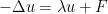 $-\Delta u = \lambda u + F$ on a ball B(0,R) in terms of the H^1 norm of u and the L^2 norm of F on this ball. In principle, this gives the uniform control on the infinitesimal rate of change $\dot u$ that we need, but only in the interior of the triangle. With reflection (and dealing somehow with the inhomogeneous Neumann conditions) one should also be able to handle things at the edges, but I haven’t thought in detail about this yet.
        
        Comment by Terence Tao — June 27, 2012 @ 1:05 am | Reply
        
        I think I can also get a Sobolev type lemma at and near vertices, allowing one to get L^infty control on the first variation $\dot u_2$ as a consequence of the L^2 and H^1 control. The idea is to work in logarithmic coordinates around a vertex (which we place at the origin), rewriting the eigenfunction u as $v(s,\theta) := u(e^s,\theta)$ (where the $(e^s,\theta)$ is interpreted in polar coordinates). This is a conformal change of variables, mapping the triangle to a half-infinite portion of a strip $\{ (s,\theta): s \in {\bf R}, 0 < \theta < \alpha \}$ , and the eigenfunction equation $-\Delta u = \lambda u$ becomes the weighted eigenfunction equation $-\Delta v = e^{2s} \lambda v$ . (But the Rayleigh quotient $\int |\nabla u|^2$ stays essentially unchanged, becoming $\int |\nabla v|^2$ . The first variation $\dot v$ of the transformed eigenfunction obeys a similar equation, basically 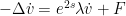$-\Delta \dot v = e^{2s} \lambda \dot v + F$ for some explicit forcing term F, together with an inhomogeneous Neumann boundary condition $\partial_\theta \dot v = f$ for $\theta = 0,\alpha$ and some explicit function f. As the domain is locally just a strip, one can easily reflect to a domain roughly resembling a half-plane with a wavy boundary, with the reflected version of $\dot v$ having an explicit Laplacian that includes some singular distributional components on the boundary of the strip (coming from the Neumann forcing term f). It looks like one can then use the fundamental solution of the Laplacian in the plane to give L^infty control on $\dot v$ and hence on $\dot u$ using L^2 and H^1 control of $\dot v$ and of f and F, with effective constants.
        
        The upshot of all this is that one should be able to get an effective version of the Banuelos-Pang stability theory (that asserts among other things that eigenfunctions react continuously in the L^infty topology with respect to changes in the domain), in all regions of the triangle (interior, edges, vertices). Not yet sure how nice the explicit constants are going to be, though.
        
        Comment by Terence Tao — June 28, 2012 @ 10:00 pm | Reply
        
        excellent, and I’m looking forward to the details. Presumable your bounds will have explicit constants involving the opening angles at the corners, right? And are you conformally mapping the triangle (Schwarz-Christoffel), or the logarithmically scaled region near the vertex? In either case, the mappings will contain angle-dependent information which would be great.
        
        I’ve talked to a few PDE numerical analysts this week about the problem, and hopefully some will comment here. In particular, Markus Melenk has significant expertise in approximation for corner domains.
        
        Comment by nilimanigam — June 29, 2012 @ 6:26 pm | Reply
        
        I started some computations at http://michaelnielsen.org/polymath1/index.php?title=Stability_of_eigenfunctions#Sobolev_inequalities_in_logarithmic_coordinates , focusing initially on the task of getting L^infty bounds on eigenfunctions near a corner. This became a little messier than I had anticipated, but the constants are still in principle explicit.
        
        The logarithmic map $z \mapsto \log z$ (or, in real coordinates, $(r \cos \theta, r \sin \theta) \mapsto (\log r, \theta)$ ) is conformal, but it isn’t of Schwartz-Christoffel type; it maps the triangle to a half-infinite strip with two parallel half-infinite edges and one bounded concave edge. The angle of the vertex becomes the width of the strip. Incidentally, it seems to me that the concavity of the edge should be somehow related to the hot spots conjecture at the other two vertices, as it makes it clearer that those two vertices ought to be acting “extremally” somehow (but I am not able to make this intuition precise).
        
        In principle the computations I gave will also extend to the inhomogeneous eigenfunction equation that shows up when taking the first variation of an eigenfunction with respect to perturbations, but the computations are getting a bit messy. But at least there are no Bessel functions involved in this approach…
        
        Comment by Terence Tao — June 30, 2012 @ 5:11 pm | Reply
        
        Thanks, the notes are helpful!
        Staring at your calculations, I asked myself the following naive question. Suppose we have a triangle with angles $\alpha, \beta, \gamma$. Using the logarithmic change of coordinates around the three corners in turn, the estimates A.7-A.13 in your notes seem to give control on the norms of the eigenfunctions in terms of both $R$ (distance from corner) and the angle.
        
        Suppose I fix $R$. Don’t A.11 and A.12 give tell us which of the three corners will have the largest mean (in the sense of $\bar{v(s)}$? In other words, don’t your calculations seem to tell us which 2 corners to focus on?
        
        Turning this around, suppose I fix a constant $C>0$ and the $R$, and ask: from A.11-12, we can roughly compute the $s$ for each corner such that the bound on $|\bar{v}(s)|$ first exceeds C. For which corner is this the smallest? This
        is the corner which will ‘concentrate’ the eigenfunction. Of course the answer will depend on the eigenvalue.
        
        To see if there was a simple answer, I wrote up a little Matlab script:
        http://www.math.sfu.ca/~nigam/polymath-figures/bound.m
        
        I fix $R=0.5$, and first pick some value of $\lambda$ (I realize this is NOT the right thing to do, but I wanted to get a feel for the bound). The script looks at the bound on the RHS of A.12 for all three angles, to see if there’s a monotonicity there. It also varies lambda, and examines the behaviour of the bound in the lambda-s parameter space.
        
        If, say, we take pi/2 and pi/3 as two of the angles, and choose a lambda larger than 10, the bounds are well-seperated and monotone in the angle as one changes s.
        
        On the other hand, for smaller lambda values these curves can cross.
        
        Now, of course all of this looks at an upper bound, and at values which are patently not the eigenvalue. But these plots gave me some insight: the question of monotonicity of the local behaviour in angle is a somewhat delicate one! It has also been extremely useful while thinking about how to do rigorous numerics: once we have a very good estimate on the eigenvalue, one looks at these bounds, and decides around which vertex to allocate a lot of grid points to sample the eigenfunction on, to locate extrema.
        
        I think this is related to your observation about the extremal nature of the vertices
        
        Comment by nilimanigam — June 30, 2012 @ 9:59 pm
        
        I should perhaps point out that in the case of the homogeneous eigenfunction equation $-\Delta u = \lambda u$ , one can solve for $\bar{v}$ exactly using Bessel functions, to obtain 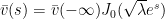$\bar{v}(s) = \bar{v}(-\infty) J_0(\sqrt{\lambda} e^s)$ ; in particular, $|\bar{v}|$ attains its maximum at $-\infty$ (incorrectly labeled as 0 in a previous version of the wiki notes). So the estimates in the wiki notes are not optimal, but the point is that they should also carry over without too much difficulty to the inhomogeneous case which is needed to control the first variation of the eigenfunction (but I haven’t done that yet).
        
        Comment by Terence Tao — July 1, 2012 @ 6:55 pm
This is in response to a comment you made on the previous thread.

I’ve put a picture of the $\alpha=\frac{\pi}{3}, \beta= \frac{\pi}{9}, \gamma = \pi-\alpha-\beta$ triangle I used to generate the data in the ill-fated file. http://www.math.sfu.ca/~nigam/polymath-figures/triangle.jpg

Clearly, not only did I have a bug (which you helped catch), I was working on the wrong triangle!! Now this is all truly embarrassing. A large part of this was my not generating actual graphics, which would have helped me catch errors.

Back to the drawing board. I’m just going to throw out this code and start again, this time generating pictures. Apologies all around.

Comment by Nilima Nigam — June 26, 2012 @ 2:55 am | Reply
- Maybe we should settle on something with nicer coordinates, see post above.
  
  Comment by Bartlomiej Siudeja — June 26, 2012 @ 3:10 am | Reply
  - I’ve sent you the source code off-line. Sure, let’s try a triangle with rational coordinates. Any preference?
    The data file has been updated as well.
    
    Comment by Nilima Nigam — June 26, 2012 @ 3:30 am | Reply
    - (0.7,0.6) is close to 40-60-80 and has simple coordinates. We could also try 45-60-75, not rational, but nice trig values, and a lot of good reflections.
      
      Comment by Bartlomiej Siudeja — June 26, 2012 @ 4:32 am | Reply
      - 1) For the 45-60-75 triangle, the coordinates of the third corner are: aa=+6.3397459622e-01, bb=+6.3397459622e-01.
        The first nonzero neumann eigenvalue I get is approximately 17.84929, and the extrema occur on the vertices.
        
        Data is at http://www.math.sfu.ca/~nigam/polymath-figures/Scalene1.odt
        Picture of first nonzero neumann eigenvalue is http://www.math.sfu.ca/~nigam/polymath-figures/45-60-75.pdf
        Looking at the contour lines one can (numerically) see there are no interior extrema.
        
        2) For the triangle with a (0.7,0.6) corner, the first neumann eigenvalue I get is approximately 17.201366077. The extrema occur on the vertices.
        
        Data is at http://www.math.sfu.ca/~nigam/polymath-figures/Scalene2.odt
        Picture of first nonzero neumann eigenvalue is http://www.math.sfu.ca/~nigam/polymath-figures/07-06.pdf
        Again, the contour lines suggest there are no interior extrema.
        
        Sanity checks would be very welcome.
        
        Observation: from most of the figures of the eigenfunctions, it can be seen that their behaviour is predominantly by that of the Bessel functions multiplied by cosines, centered around the corners. That is, as asymptotics would suggest, near a corner the eigenfunction looks like that of a sector; however, the asymptotics seem valid rather far from the corner.
        
        Indeed, I’d think if one subtracts a linear combination of these functions from the eigenfunction, what’s left looks almost like a ‘bubble’- nearly zero on the bulk of the boundary, and a little bumpy in the middle.
        
        Comment by Nilima Nigam — June 26, 2012 @ 8:12 pm | Reply
        
        It seems that the files are 403’ed (i.e. not publicly accessible).
        
        Comment by Terence Tao — June 26, 2012 @ 8:20 pm | Reply
        
        should be fixed now.
        
        Comment by Nilima Nigam — June 26, 2012 @ 9:58 pm | Reply
        
        Thanks! I can access the files now.
        
        The contours in these images look like they are giving some monotonicity properties on the eigenfunction, but we know unfortunately that this is not exactly the case – something funny happens near the vertex opposite the longest side, and also when the triangle is nearly sub-equilateral isosceles we know that the eigenfunction should be nearly symmetric around the near-axis of symmetry, and so would not have monotonicity on the approximate base of this nearly isosceles triangle. This is a pity – ideally there should be some monotonicity-type property that one could see by inspection from the contour plots of various acute triangles which might be easier to prove (either theoretically or numerically) than directly hunting for the location of extrema, and which would imply something about those extrema. At present though I do not have a candidate for such a property that isn’t ruled out by looking near vertices or near the isosceles cases.
        
        Comment by Terence Tao — June 26, 2012 @ 11:26 pm | Reply
        
        For both triangles I get exactly the same numbers, and global extremum at the vertex straddled by the nodal line. One thing I cannot find is circular level lines around the vertex opposite longest edge. I guess its contribution in linear combination of Bessel functions is extremely small (equal 0 for super-equilateral triangles).
        
        Comment by Bartlomiej Siudeja — June 26, 2012 @ 9:14 pm | Reply
        
        yes! I think this coefficient in the linear combination must be small. Here is what I observe, based on crude numerics:
        
        if i write $u(x,y) = c_1 \phi_1(x,y) + c_2 \phi(x,y) + c_3\phi(x,y) + l.o.t.$, where $\phi_i$ is the Bessel-Fourier basis function for the ith vertex, then the coefficient $c_k$ corresponding to the vertex opposite the longest side (ie, $\phi_k$ corresponds to the widest angle) is the smallest in magnitude of the three $c_j$.
        
        Comment by Nilima Nigam — June 26, 2012 @ 10:03 pm | Reply
        
        Is it possible to get good bounds for eigenvalue/eigenfunction from the generalized fundamental solution method in terms of how far from 0 Neumann condition is on the boundary of approximate eigenfuntion? Something like FHM for Dirichlet condition.
        
        Comment by Bartlomiej Siudeja — June 26, 2012 @ 11:04 pm | Reply
        
        this is exactly the spirit of what I implemented — the method of particular solutions of Betcke and Trefethen etc. Unfortunately, as far as I know, there is no proof of error control for the Neumann problems on non-domains yet. So I’m reluctant to rely on these numerics.
        
        Comment by Nilima Nigam — June 27, 2012 @ 2:25 am | Reply
        
        What do you mean by non-domains? This method is great for getting numerical results, most likely better than FEM, especially for triangles It would be great if there was actual error bound. Assuming we/someone could prove one, bounds for gap and second eigenvalue will tell us if the eigenvalue we are converging to is second or third.
        
        Comment by Bartlomiej Siudeja — June 27, 2012 @ 4:01 am
That should be non-smooth domains.

I agree it seems to give great results, but remain wary of posting anything based on a method about which I can’t prove convergence. I think we can safely conclude, from the FEM calculations, that we’re getting the second eigenvalue. The MPS method in principle helps us get better accuracy.

I’ll try to ask some people who may know about MPS.

Comment by Nilima Nigam — June 27, 2012 @ 4:35 am | Reply
- This might be a stupid question, but is it known that FEM is not missing any eigenvalues? In any case, whatever we are getting as numerical eigenvalue, we can show this is not the third eigenvalue by using a lower bound for the third eigenvalue (or gap bound and second eigenvalue bound). This could be especially important near equilateral triangle, where the eigenvalues are really close.
  
  Comment by Bartlomiej Siudeja — June 27, 2012 @ 4:54 am | Reply
  - This is a very good question. I break up my answer in two parts:
    
    1. Suppose we had an *exact* method for doing the linear algebra for a discrete system.
    
    We ask: as an approximation problem, will the FEM solutions converge to the true one?
    
    After writing the continuous eigenvalue in discrete form (ie, making the matrices), for the Laplace eigenvalue problem the H1-conforming finite element method will converge, and there are rigorous bounds. The spectrum is accurately captured, especially for the smaller eigenvalues.
    
    It’s the curl-curl system for which one needs to be very careful.
    For a very nice talk by Boffi on this, see http://www.ann.jussieu.fr/hecht/ftp/Ecole-Cirm-EFEF5/boffi/boffi1.pdf with the sketch of the proof for piecewise linears. A good exposition on a posteriori error estimation is by Vincent Heuveline and Rolf Rannacher.
    
    2. Suppose we are given a large discrete eigenvalue problem $Ax =\lambda B x$ to solve.
    
    There is no *exact* method for computing the eigenvalues of a large system. Therefore, one does something iteratively.
    
    If one knew nothing about the structure, I believe there is no proof the Arnoldi iteration would give the correct eigenvalues. However, since we cleverly picked a conforming method in 1), and our system is symmetric, Arnoldi reduces to the Lanczos iteration. It is implemented in its stable form. The eigenvalues converge to those of the original system.
    
    In the case of the Neumann eigenvalues, it is safer to introduce some kind of shift.
    
    Now, we put these together. We will see the impact of rate of convergence of the different FEM, as well as the Lancoz method’s abilities, in the following. I did this for the equilateral triangle, which is hard (because of the multiplicity).
    
    Piece-wise linear polynomials
    
    aa=+5.0000000000e-01 bb=+8.6602540378e-01alpha=+1.0471975512e+00beta =+1.0471975512e+00gamma=+1.0471975512e+00scaled min Corner1 Corner2 Corner3
    #DOF = Eigenvalue1 EV2 EV3
    +64 +1.7767788818e+01 +1.7785194621e+01 +5.4705187554e+01
    +226 +1.7601919340e+01 +1.7602672236e+01 +5.3122837928e+01
    +845 +1.7560008052e+01 +1.7560403267e+01 +5.2763327020e+01
    +3264 +1.7549418792e+01 +1.7549447033e+01 +5.2668553766e+01
    
    Note the slow convergence at this stage. The linear algebra fails to detect the multiplicity for this low-order method on a coarse mesh, and the finite element method is converging only linearly. After 4 iterations we have only 4 digits of accuracy.
    
    Piece-wise quadratic polynomials
    
    aa=+5.0000000000e-01 bb=+8.6602540378e-01alpha=+1.0471975512e+00beta =+1.0471975512e+00gamma=+1.0471975512e+00
    #DOF = Eigenvalue1 EV2 EV3
    +223 +1.7546517328e+01 +1.7546602541e+01 +5.2654106745e+01
    +841 +1.7545997420e+01 +1.7545999345e+01 +5.2638899549e+01
    +3257 +1.7545965667e+01 +1.7545965754e+01 +5.2637955725e+01
    
    The 2nd-order FEM is doing better. After 3 refinements, we have 6 digits of accuracy in the eigenvalue. The Lancoz method is starting to demonstrate that the first and second eigenvalues are close (to 9 digits).
    
    Piece-wise cubic polynomials
    aa=+5.0000000000e-01 bb=+8.6602540378e-01alpha=+1.0471975512e+00beta =+1.0471975512e+00gamma=+1.0471975512e+00
    #DOF = Eigenvalue1 EV2 EV3
    +478 +1.7545964458e+01 +1.7545964540e+01 +5.2637977206e+01
    +1846 +1.7545963396e+01 +1.7545963397e+01 +5.2637891423e+01
    +7237 +1.7545963380e+01 +1.7545963380e+01 +5.2637890161e+01
    +28648 +1.7545963380e+01 +1.7545963380e+01 +5.2637890139e+01
    
    The 3rd order FEM is great. After 4 iterations we have 11 digits of accuracy in the eigenvalues. Correspondingly, the Lanczos method also picks up on the repeated eigenvalue: it reports they are close for the coarsest mesh (to 8 digits), and that they are identical to 10 digits by the 3rd mesh.
    
    The moral of the story is: these work-horse methods (conforming FEM+Lanczos) are provably convergent, and give good results if used carefully.
    
    Comment by Nilima Nigam — June 27, 2012 @ 1:30 pm | Reply
Continuing the discussion, I now present results for the nearly equilateral triangle with $\frac{pi}{3} – 0.00001, \frac{\pi}{3}, \frac{pi}{3} + 0.00001$. Sanity checks would be helpful, but I think I’m working on the correct triangle.

This time, I present only at the results using piecewise cubic elements, and the computed spectral gap. First, looking down the columns for EV1 or EV2, you see convergence to 10 digits. The spectral gap is of magnitude 3.6e-04. In other words, the difference between the computed eigenvalues 17.545985982630999 and 1.7546345986811367 occurs in the 4th digit after the decimal. The eigenvalues are converged to 9 digits after the decimal. One can assert that in the limit as we refine the mesh more and take more Arnoldi iterations, this difference will persist.

Piece-wise cubic polynomials
aa=+5.0000577346935882e-01 bb=+8.6601540384217246e-01alpha=+1.0471875511965976e+00beta =+1.0471975511965976e+00gamma=+1.0472075511965977e+00
#DOF = EV1 EV2 EV2-EV1
+505 +1.7545986801305649e+01 +1.7546346667927342e+01 +3.5986662169307237e-04
+1936 +1.7545985995561395e+01 +1.7546345999012988e+01 +3.6000345159337144e-04
+7462 +1.7545985982843547e+01 +1.7546345986984758e+01 +3.6000414121062363e-04
+29278 +1.7545985982630999e+01 +1.7546345986811367e+01 +3.6000418036863380e-04

Comment by Nilima Nigam — June 27, 2012 @ 3:07 pm | Reply
Here’s a nice paper on error estimates for FEM approximations of the Dirichlet problem (not the eigenvalue problem!) in various norms, including results in the sup-norm: http://imajna.oxfordjournals.org/content/26/4/752. In the method discussed both the size of triangles (h) and the polynomial approximation (p) can vary. Theorem 2.1 is the main result.

I am still looking around for the equivalent results for eigenvalue computations. The regularity of eigenfunctions one can expect is similar to those assumed in this paper, but the arguments in the proof may be different.

Comment by Anonymous — June 30, 2012 @ 3:56 pm | Reply
The file I posted in comment (2) http://www.math.sfu.ca/~nigam/polymath-figures/bound.m, and the two graphs, have been changed to have logarithmic coordinate $s$ run in the correct interval. The behavior of the bounds is switched.

Comment by Anonymous — July 1, 2012 @ 10:26 pm | Reply
A small observation (that came up while doing the Sobolev bounds): if $u$ is a Neumann eigenfunction ( $-\Delta u = \lambda u$ ) on a triangle ABC, with a vertex A at the origin, then the angular derivative $\partial_\theta u$ of that eigenfunction becomes a partially Dirichlet eigenfunction on that triangle, as that derivative also obeys the eigenfunction equation $-\Delta \partial_\theta u = \lambda \partial_\theta u$ (this can be seen by looking at the Laplacian in polar coordinates, or by using the rotational symmetry of the Laplacian) and (because of the Neumann boundary condition on u) vanishes on the two sides AB, AC (but does something weird on the far side BC). I don’t know how to make more use of this observation though.

Comment by Terence Tao — July 3, 2012 @ 6:36 pm | Reply
- What comes to my mind is the fact that $\partial_\theta u = 0$ implies that the level curves of $u$ are circles. So maybe somehow getting rigorous bounds on $\vert\partial_\theta u\vert$ could give some control on the shape of the level curves– i.e. that they are almost circles.
  
  Of course the only place I see a clear argument is close to a corner (which is then near to two Dirichlet boundaries)… but for corners we already know that the level curves are concentric circles.
  
  If we consider the case of a triangle all of whose corners are local extrema (I think most of the triangles we still need to worry about are this case?), then there is the following observation: Suppose the triangle has one hot corner $A$ and two cold corners $B$ and $C$ and orient the triangle as in the parent comment. Then in addition to having the two Dirichlet boundaries $AB$ and $AC$ , we also have that $\partial_\theta u$ achieves both positive and negative values on $BC$ …. which makes it plausible that $\partial_\theta u$ is closer to $0$ in the interior… which in turn implies that the concentric circular level sets around $A$ extend farther into the interior than those of $B$ and $C$ . This matches the simulated eigenfunctions also. But this is a cheating argument since I am already assuming much about the structure of the second eigenfunction :-)
  
  ——
  As a side note, while before I had conjectured that “For a convex domain, one of the nodal domains should be convex” I now don’t think that is true: I believe that a long and narrow parallelogram would have an S-shaped nodal line.
  
  Comment by Chris Evans — July 3, 2012 @ 9:27 pm | Reply
  - In fact almost any parallelogram should have S-shaped nodal line. Any parallelogram has 2-fold rotational symmetry, hence its eigenfunction must also be 2-fold symmetric. Since nodal line starts perpendicular to the boundary and goes through the center, it must be either a straight line (rectangles) or have some sort of S-shape (generic parallelogram). It is also possible that nodal line starts at a vertex, but this most likely means that we have a rhombus (the line is also straight in this case). I am not sure how to prove those claims but numerical results agree with the above. For parallelogram with vertices (0,0), (1,0) and +-(0.55,0.45) one gets a really nice S-shape, even though the domain looks almost like a square. Even squares have S-shaped nodal lines if you choose a wrong eigenfunction (eigenvalue is doubled).
    
    Comment by siudej — July 5, 2012 @ 5:32 am | Reply
    - Good point about the symmetry… that is a more rigorous argument than what I had in mind.
      
      I have this strange picture in my head for visualizing the nodal line:
      
      I imagine a “red army” started from a point mass of +1 at some point $x$ and a “blue army” started from a point mass of -1 at some point $y$ . Then as time evolves the armies diffuse and where they meet they destroy each other. Then in the long run, the nodal line is the “battle line” between the two armies.
      
      From this perspective it seems plausible that the nodal/battle line for a parallelogram would be an S-shape: There would be, say, more of a push from the red army in the north and the blue army in the south. And for a triangle it would seem plausible that the nodal line looks like an arc: The red army is confined to a corner pushing outward.
      
      This interpretation also gives a characterization of the extrema of the second eigenfunction: They are the points where you would start the “two armies so that both armies last the longest”. This is certainly true if you measure “army size” by the L^2-norm, and it should be true for other L^p-norms as well (in the long run the distribution looks like the second eigenfunction and we can use that to convert between norms without needing constant factors) In particular, since the L^1-norm is equal to the total variation distance (think now of the red and blue armies as the distributions of two reflected Brownian motions started from $x$ and $y$ )… it should be possible to give a characterization of the extrema as: The points you would start two random walkers such that they take the longest time to couple under an optimal coupling (i.e. a minimax statement). [This is stuff I have been working on before but haven’t gotten around to writing up]
      
      But while these interpretations give some intuition they aren’t really useful at explicitly locating the extrema or nodal line…
      
      Comment by Chris Evans — July 5, 2012 @ 6:56 pm | Reply
I managed to hack out an H^2 stability bound (i.e. the first variation of an eigenfunction has second derivatives in L^2 assuming a spectral gap), at http://michaelnielsen.org/polymath1/index.php?title=Stability_of_eigenfunctions#H.5E2_theory . But it’s very messy, I’m looking around for a better argument. The main difficulty is due to the fact that the Neumann boundary condition keeps changing when one deforms the triangle. I’m now experimenting with an older idea of using Schwarz-Christoffel transformations (using, say, the unit disk as the reference domain), the point being that a conformal transformation preserves the Neumann boundary condition. No results as yet, but I’ll keep you all posted.

Comment by Terence Tao — July 4, 2012 @ 1:38 am | Reply
- OK, the H^2 theory is _much_ cleaner in the Schwarz-Christoffel framework. (Sorry for switching in and out of different formalisms; it’s taking a while to find the most natural framework in which to do all this.) Details are at http://michaelnielsen.org/polymath1/index.php?title=Stability_of_eigenfunctions#H.5E2_theory . Basically, the Schwarz-Christoffel strategy is to (temporarily) use the _half-plane_ as the reference domain, rather than a triangle, using Schwarz-Christoffel transformations to do the change of coordinates. The transform itself is given by an integral, but the derivative of the transform is an explicit rational function, and this turns out to be the more important quantity. The advantages of this are (a) the Schwarz-Christoffel transformations are conformal and thus preserve the Neumann condition (and modify the Laplacian by a conformal factor e^{2\omega}), and (b) the conformal factor transforms in a nice way with respect to deformation of the angles, being multiplied by an explicit logarithmic factor. As such, one has very clean estimates for the H^2 norm of the variation $\dot v_2$ of the second eigenfunction v_2 on a triangle ABC with respect to perturbation of the angles $\alpha,\beta,\gamma$ . Basically, one has
  
  $(\int_{ABC} |\nabla^2 \dot v_2|^2)^{1/2} \leq \frac{4\lambda_2 \lambda_3}{\lambda_3-\lambda_2} (\int_{ABC} |\dot w|^2 |v_2|^2)^{1/2}$
  
  where $\dot w$ is the variation of the conformal factor, which blows up like log |x-A| around the vertex A and similarly at B and C (and can be written down explicitly). Because the logarithm blows up so slowly, it should be a relatively straightforward manner to control the integral on the RHS in terms of, say, the H^1 norm of v_2; combining this with a suitable Sobolev inequality on the triangle, one should be able to get pretty good L^infty bounds on the variation of the eigenfunction. I might try this first for the 45-45-90 triangle where things should be fairly explicit.
  
  Comment by Terence Tao — July 4, 2012 @ 7:17 pm | Reply
  - Excellent news! It seems rather natural to use the Schwarz-Christoffel map, since it deals with all the corners in one shot. Indeed, if this attack works, it may point the way for the Hot Spot conjecture on more general domains as well – anything for which a conformal map to the upper half plane exists.
    
    With these bounds within reach, here is the outline of a numerical strategy.
    
    – Place a ‘mesh’ on parameter space of angles. The spacing of the grid points should be such that r-neighbourhoods of these grid points cover the space of interest. r is to be chosen so we are confident that the behaviour of eigenfunctions for triangles in an r-neighbourhood are well-controlled in terms of the behaviour of the spectral gap and eigenfunction at the grid point. For example, one of the (several) criteria to use in choosing ‘r’ is that the eigenfunctions will not vary by more that $\epsilon>0$ in the sup norm.
    
    – At each grid point in parameter space, use only provably convergent algorithms to compute approximations to the eigenfunction, detailing all the approximations involved. Ensure the resultant approximation is within $\epsilon/(10 r)$ or some such safety factor in the sup norm. We now know corners are local extrema; the nodal line theorem will prohibit oscillations on a fast scale. If the extrema of the computed eigenfunctions are on the corners on highly refined grids, and if the hot-cold values are well-seperated, I think one will be able to conclude the results.
    
    I have to digest the bounds in your argument a bit, before I attempt to implement the above strategy.It may be we need to choose different ‘r’ values in different regions of parameter space. The spectral gap is rather small near the equilateral triangles, but previous arguments seem to indicate there’s a good handle on this area anyway.
    
    It would be optimal if several people were to independently do these calculations using the same standards and the same grids, but using different architectures and software.
    
    I tried a coarse variant of this approach for the earlier figures I posted, and it’s tractable. I think we’ll be limited to lower-order methods. Regrettably, the method of particular solutions (Betcke/Trefethen) is efficient, but there is no proof yet that it converges for the Neumann problem on polygonal domains. So at best it should be used as a sanity check.
    
    Comment by nilimanigam — July 5, 2012 @ 2:45 am | Reply
    - I can try to replicate your numerical results using my scripts. By lower order do you mean order 1? Cubics are really nice and do not require really fine mesh.
      
      Comment by siudej — July 5, 2012 @ 5:41 am | Reply
      - That would be great! I think we should try with 1st, 2nd and 3rd order polynomials, but no higher. The 3rd order polynomials give good convergence on even a rather coarse mesh, but then we have to interpolate onto a truly fine mesh to locate the extrema with reliability. The first order nodal elements need a very fine mesh, but then there’s no interpolation necessary. This was we have different kinds of control on the method of finding the actual extrema.
        
        Comment by Anonymous — July 5, 2012 @ 2:42 pm | Reply
  - I managed to find a reasonably nice Sobolev inequality (basically based on the elementary Sobolev inequality that controls L^infty by W^{2,1} in two dimensions by two applications of the fundamental theorem of calculus) which gives a completely explicit stability theorem in L^infty in Schwarz-Christoffel coordinates; details are at http://terrytao.files.wordpress.com/2012/07/perturbation.pdf . The constants involve gamma functions, the second and third eigenvalue, and a certain explicit integral on the half-plane of a rational function multiplied by a logarithmic factor, so in principle we can compute (or at least bound) it with what we have.
    
    Comment by Terence Tao — July 6, 2012 @ 1:54 am | Reply
    - This is very handy, thanks!
      
      I think the bound will be useful. Some quantities in it will need to be approximated – we won’t have the eigenvalues exactly for most triangles. However, I think the bound you derived can be approximated from above, given how the spectral gap enters in the bound.
      
      In the absence of the actual eigenvalues, we’ll be using approximations of the form $\lambda_{k,h}$ where $h$ is some discretization parameter. Most of the error bounds look like $|\lambda_{k,h}-\lambda_{k}| \leq C_k h^{r}$, where the $C_k$ depends on the spectral gap. I think that Still’s arguments, with suitable modifications for the Neumann case, will be handy.
      
      The bound you derived is also useful in terms of thinking about where, in parameter space, we may consider very fine sampling. The spectral gap $\lambda_3-\lambda_2$, scaled by the area of the triangle, is small near the equilateral triangles. It also appeared to be getting small for triangles in which one angle is small.
      
      Comment by nilimanigam — July 6, 2012 @ 4:13 am | Reply
      - One small angle means 2 sides are nearly perpendicular. Hence eigenfunctions should be like for a rectangle, 2 or three nodal lines in one direction. You can make a rectangle arbitrarily thin without changing eigenvalues. So eigenvalues stay the same, while area goes to 0. This indicates that area is not a good scaling factor for Neumann eigenvalues. It would be perfect for Dirichlet. For Neumann it is more reasonable to use diameter scaling. At least this way you are not running into this weird fixed eigenvalue, decreasing scaling factor scenario. In fact diameter appears in Poincare inequality.
        
        Same happens for thin sectors, where radial eigenfunctions are better than adding trigonometric factor.
        
        Comment by siudej — July 6, 2012 @ 6:00 am | Reply
        
        This makes sense! I’ll revisit those calculations.
        Since the $L^\infty$ bounds just derived depend explicitly on the spectral gap, I’ll also keep track of the unscaled quantities.
        
        Comment by nilimanigam — July 6, 2012 @ 2:20 pm | Reply
      - One small remark: I had an integral (denoted $\int_H |\dot \omega|^2 e^{2\omega}$ in my notation) that showed up in the stability estimate which I thought had no closed form expression, but I have since realised that it is just (one quarter of) the second derivative of the area function $\int_H e^{2\omega} = |ABC|$ in time and so does have a closed form (but messy) expression in terms of Gamma and trig functions and their first two derivatives. I wrote up the details at http://terrytao.files.wordpress.com/2012/07/perturbation1.pdf (basically a slightly edited version of the previous notes), though I didn’t bother to fully expand out the second derivative as it was somewhat unenlightening. (I should at least work out what the stability estimate is doing in the 45-45-90 case, though, where everything is explicit, but I’m too lazy to fire up Maple and evaluate all the constants..)
        
        Comment by Terence Tao — July 6, 2012 @ 9:47 pm | Reply
        
        In an attempt to compute the constant X, I pulled back the variation of the conformal factor $\omega$ to ABC. I got a horrendous expression, but a quick comparison of leading terms suggests it’s the same as the variant you have.
        
        My goal is to end up with something which can be computed via quadrature on ABC.
        
        I had a question, though, based on ignorance about the smoothness properties of the perturbations.
        
        When we vary the angles smoothly, do the eigenfunctions vary in the time variable in a C^1 fashion? Staring at how the nodal lines move around as one varies the angles, I can somewhat convince myself of this for triangles which are far from isoceles or equilateral. I’m less certain about the situations where we move away from isoceles.
        
        In your argument I believe you use this smoothness only in the step where you formally differentiate, (2.7).
        
        If instead one uses a discrete change $\tilde{u} \rightarrow \tilde{u} + \delta u$ , and correspondingly $\lambda\rightarrow \lambda+\delta \lambda$ , (2.7) will change a bit. The middle term gets replaced by $\lambda \tilde{u} (e^{2\delta \omega}-1)$ , which in limit of smooth deformations reduces to what you have. For the other terms one gets quantities in terms of $\delta \lambda$ and $\delta u$ . I think the string of identities (2.8-2.9) remains true, and the rest of the argument should be fine as well. Since we want control on the discrete variation, but not on its first time-derivative, this should be OK, right?
        
        Comment by nilimanigam — July 6, 2012 @ 10:23 pm | Reply
        
        I expect to have C^1 regularity of the variation as long as there is a spectral gap. In the first L^2/H^1 stability notes in http://michaelnielsen.org/polymath1/index.php?title=Stability_of_eigenfunctions#L.5E2_and_H.5E1_theory (which is based on discrete variation rather than continuous variation), it is shown that the second eigenfunction behaves in a locally Lipschitz manner in the L^2 and H^1 metrics with respect to the angle parameters, so long as there is a spectral gap (i.e. one is not equilateral). (Admittedly, this is using a fixed triangle as the reference domain, rather than the half-space, but I think that this is not a significant obstacle.) I believe that with a little more work one can upgrade “Lipschitz” to “differentiable”, with the derivative being given by the formal variation formula appearing in the notes. The formal variation itself varies continuously even in the H^2 topology, so then the fundamental theorem of calculus (when applied carefully) should then show that the eigenfunctions are C^1 in the H^2 topology. I can try to work out the details of this over the next few days and write it up.
        
        Comment by Terence Tao — July 6, 2012 @ 11:01 pm | Reply
        
        OK, I wrote up the details (modulo some handwaving involving Hardy’s inequality which I was too lazy to do in detail) at http://terrytao.files.wordpress.com/2012/07/perturbation2.pdf . In that file I also tried working out what the explicit bound is for the C^0 variation bound $\| \dot u_2 \|_{L^\infty} \leq X \| u_2 \|_{L^\infty}$ in the explicit example when one is perturbing a 90-45-45 triangle by keeping the right-angle $\alpha=\pi/2$ fixed and increasing the second angle $\beta=\pi/4$ at rate 1 (and thus decreasing the third angle $\gamma = \pi/4$ at the opposite rate -1). I (or more precisely, MAPLE) got X = 22.34 when doing this (but this may bear some double-checking), which roughly speaking means that one can perturb the angle beta by about 1/20 or so before losing all control on the extrema. So the bounds are feasible enough that the mesh idea might actually work. (One might also do some numerical exploration of what $\|\dot u_2 \|_{L^\infty}$ actually is, to get some idea of how inefficient the bounds in that file actually are, and whether there is much scope for further improvement.)
        
        There are of course some additional issues to work out. The first is that L^infty control on the perturbation does not quite, by itself, tell us where the extrema go; one also needs the eigenfunction to stay some fixed distance away from the extrema away from the vertices, and to obey some quantitative non-degeneracy at and near the vertices. I think I can hack out something about the latter using Bessel function asymptotics, but the former will need numerics. I guess I could go look at the 90-45-45 triangle again where everything is explicit…
        
        Comment by Terence Tao — July 10, 2012 @ 12:29 am | Reply
        
        I’m currently coding up the following.
        
        I’ve also been thinking about how I’d examine the variation in the eigenfunctions, since nominally these are computed on different geometries. It’s computationally easier to pull everything back to a finite reference right triangle.
        
        1) On a coarse mesh in parameter space, pick triangles of base 1 either whose third vertex has rational coordinates, or whose angles are rational multiples of pi.
        
        2) On each point in parameter space, compute the 2nd and third eigenvalues and eigenfunctions. I also compute the right hand side of the bound in your previous notes (suitably scaled, since the Schwarz-Christoffel map did not map to a triangle of base 1). Map the eigenfunctions to the reference right-angled triangle.
        
        3) Take a small linear ‘time-step = $\delta$ ‘ in the alpha angle, keeping beta fixed. Compute the second eigenfunction on the new triangle with base 1 and $\alpha+ \delta, \beta, \gamma-\delta$ . Pull this back to the reference right-angled triangle. Compare with the eigenfunction obtained in step 2.
        
        4) Repeat (3) for a small linear step in the beta angle.
        
        I’m in the tedious debugging phase, and there is obvious room for improvement. For now, calculations at 5 points in parameter space suggest the upper bound is a ‘safe’ one, in that the variation stayed well controlled for a ‘time step’ of 0.01 radians. But I’m not yet confident in the code to post results yet.
        
        Additionally, for most of the eigenfunctions calculated a while ago,
        http://www.math.sfu.ca/~nigam/polymath-figures/eigen2.html
        
        the hot and cold values are well-separated. (Clicking on the triangles should show the values of the colorbars). This does not imply, necessarily, that the eigenfunctions cannot become flatter. But in the ‘eye-ball’ norm, the regions away from the corners are rather far from being hot or cold.
        
        Comment by nilimanigam — July 10, 2012 @ 1:01 am | Reply
        
        Sounds like it should basically be a workable approach. One slight issue is that an L^infty stability result in the Schwarz-Christoffel coordinates doesn’t immediately imply an L^infty stability result in the affine coordinates, unless one also uses some sort of C^1 bound on the eigenfunction in order to control the error between the two different coordinate systems in L^infty. (I ran into this issue when trying to pass between differentiability of the eigenfunction in time in affine coordinates, to in Schwarz-Christoffel coordinates; it seems that changing coordinates tends to lose one degree of regularity in space in the time derivative.)
        
        One thing which isn’t in the current stability notes, but which I will try to put it at some point, is some sort of stability estimate for the spectral gap. If we have one triangle where we know a quantitative gap between lambda_2 and lambda_3, then there should be an explicit estimate that gives a similar gap for all nearby triangles. (Presumably some variant of Siudeja’s arguments would work to give this.) This means that the stability constant X in my notes should itself be stable with respect to small perturbations, so that one controls not just the time derivative of the eigenfunction, but also the error between two eigenfunctions from macroscopically distinct triangles (and hopefully at a level like the 0.01 radian scale you mentioned). (This means we also have to get some stability bounds for Gamma functions and their derivatives, as these also show up in the X quantity, but this is presumably straightforward.)
        
        Comment by Terence Tao — July 10, 2012 @ 5:23 pm
        
        Here’s what I tried in Step (2) described in Thread 9:
        
        I shrank the triangle obtained from the Schwarz-Christoffel map (ABC in your notes) by a factor of |AB| in both the x and y directions. This gives me a triangle (PQR) with base 1. I can see the potential for difficulty with the stability result (since the scaling involves |AB|, which in turn involves the angles). However, since the scaling is just a diagonal map, I thought it may be OK.
        
        Looking at the Rayleigh quotient, I think the eigenvalues on (PQR) are $|AB|^2$ times the eigenvalues on (ABC).
        The pullback of the eigenfunction itself should not change the values of its extrema. That is, I think $\|u\|_{\infty, PQR} = \|u\|_{\infty,ABC}$. In the bounding function $X$, $|ABC|\rightarrow |AB|^2 |PQR|$, the eigenvalues are appropriately scaled, and the integral over $\mathbb{H}$ remains the second derivative of the symmetric term involving the gamma functions. This integral I did not change, and compute by calling a symbolic toolbox (Maple).
        
        Is this correct? My rationale for not computing on the triangle ABC is that a finite element mesh generator would have to approximate the coordinates of 2 of the corners in terms of Gamma functions, rather than on PQR, where I’m picking corners that are rational or whose approximations which are well understood. This may be nitpicky, but I’d rather not introduce more sources of approximation errors; each has to be accounted for.
        
        Comment by Anonymous — July 11, 2012 @ 3:20 am
        
        Given quantitative spectral gap on a triangle one can surely use operator norms of affine transformations to get spectral gap for nearby triangles. Another, more complicated possibility (that I think should work) is to use triangulation argument as in the proof of simplicity. The method there does not really require explicit knowledge of the eigenfunctions on “grid” triangles. Bounds for eigenvalues on nearby “grid” triangles should be enough to get good gap estimates on any triangle. So instead of using known cases as int the proof of simplicity one could use numerically calculated bounds for eigenvalues on “grid” triangles.
        
        Comment by Bartlomiej Siudeja — July 11, 2012 @ 4:25 am
This paper by G. Still provides good bounds on the distance of approximate eigenfunctions from exact eigenfunctions, which will prove useful when trying to get exact asymptotic constants in our numerical method.

Click to access fulltext.pdf

Comment by Nilima Nigam — July 5, 2012 @ 9:59 pm | Reply
I just wrote some notes for effective Sobolev inequalities near vertices at

http://michaelnielsen.org/polymath1/index.php?title=Stability_of_eigenfunctions#Another_Sobolev_bound

Basically, it shows that near a vertex 0 of angle $\alpha$ , an eigenfunction u has the asymptotics $u(r,\theta) = u(0) J_0(\sqrt{\lambda} r) + O( r^{\pi/\alpha})$ , with effective bounds on the O() error. in principle, this allows us to exclude extrema near vertices.

Comment by Terence Tao — July 14, 2012 @ 8:01 pm | Reply
[…] Polymath7 is going strong on the polymath blog. […]

Pingback by Some Updates | Combinatorics and more — July 16, 2012 @ 5:49 pm | Reply
Here are some results. I’d be grateful if someone could double-check some of these calculations.

These graphs represent about 450 points in parameter space, with a spacing of about 0.027 radians in the $latex\alpha$ and $\beta$ directions. I’ve got a calculation with a finer spacing in parameter space running now.

As expected, the bounds on the variation become huge near the equilateral triangle, and then again near the nearly degenerate triangles. Given the range of values these bounds take on, I think a non-uniform grid in parameter space is called for.

– I’ve described the method of attack, as well as how I compute the $L^\infty$ bounds from Terry’s notes, here:

Click to access Validation+Numerics.pdf

– Graphs of the second and third Neumann eigenvalue, as a function of $\alpha, \beta$ , computed by piecewise quadratic finite elements, are here:

– The spectral gap, as well as the log of the spectral gap, as a function of $\alpha, \beta$ , computed by piecewise quadratic finite elements, are here:http://www.math.sfu.ca/~nigam/polymath-figures/SpectralGap-07.jpg

– The bounds, computed for the two cases (A): $\alpha,\gamma$ vary and $\beta$ does not, (B) $\beta,\gamma$ vary and $\alpha$ does not, are plotted here: http://www.math.sfu.ca/~nigam/polymath-figures/Boundx-07.jpg

For all of the parameter values, I also computed numerically where the extrema lie, and the spacing between them. I haven’t plotted these, but could easily do so if required. For each of these triangles the extrema of the 2nd eigenfunction occurred on the vertices.

Comment by nilimanigam — July 21, 2012 @ 3:30 am | Reply
- – I should have said that I plotted $\log(X)$ as a function of $\alpha_0,\beta_0$ , for two different cases:
  
  case 1: $\alpha(t)=\alpha_0 + t, \gamma(t)= \gamma_0-t$
  case 2: $\alpha(t)=\beta_0 + t, \gamma(t)= \gamma_0-t$
  
  There are no surprises: the bound is very large near the equilateral triangles (since the spectral gap is small) and near the nearly degenerate triangles. I did not expect the differences to be so large, however; this suggests a uniform sampling of parameter space would be very inefficient.
  
  – I’d be grateful if someone could verify some of the numbers: for the given alpha and beta (base angles), on a triangle of base 1, I get the following
  
  Alpha Beta \lambda_2 \lambda_3
  1.5437 0.0271 14.6892 49.2426
  1.5708 0.0542 14.6676 49.1703
  1.5166 0.0542 14.7107 49.3149
  1.3271 0.7854 14.0612 24.5279
  1.3541 0.8125 13.3152 22.4980
  1.3812 0.8396 12.4256 20.8035
  1.4083 0.8666 11.3990 19.4217
  1.5166 1.3541 1.0907 3.6551
  1.5437 1.3812 0.6965 2.3346
  1.5708 1.4083 0.3911 1.3111
  0.8396 0.7312 19.5933 40.1433
  
  In case there is an error, please let me know. There were several loops and index-shifting involved, so though I’ve checked, it is still possible there is a bug.
  
  Comment by nilimanigam — July 21, 2012 @ 4:37 am | Reply
Graphs computed with a grid spacing of 0.016 radians in parameter space are here:
http://people.math.sfu.ca/~nigam/polymath-figures/graphsJuly21/
The titles should be self-explanatory. I’ve included graphs of the maxima and minima of the eigenfunctions: one can see the eigenvalue solver does not discriminate between the eigenfunctions $u, -u$. A more pertinent graph concerns the difference $u_max-u_min$ of the second eigenfunction.
Once again, for all the 1273 choices of angles in this experiment, the numerical eigenfunctions attain extrema at the corners. Given how smoothly the eigenvalues, spectral gaps, eigenfunction spread and bounds vary away from the equilateral triangle, I think at least numerically the Hot Spot conjecture seems to hold.

In these calculations, the largest values of the bounds (in the alpha or beta direction) is around 8000, in the vicinity of the equilateral triangles. Of course this number is going to grow, the closer we get to the equilateral triangle. Also, the bound doesn’t grow symmetrically (ie, stepping in the alpha and beta directions change the bound differently). I think this has to do with how the second and third eigenvalues move apart, asymmetrically, in changes in the alpha and beta directions. So using the bound to calculate a good spacing in parameter space will not work near the equilateral triangle.

I have a question at this juncture. We already have some (analytic) insight into what occurs near the equilateral triangles (orange region near H in the parameter map of Terry), using perturbative ideas from Banuelos and Pang. How far away from the point (pi/3,pi/3,pi/3) do these perturbative ideas extend? In other words, how fat is the blue disk in https://polymathprojects.files.wordpress.com/2012/06/triangle31.png? If we can excise this disk from parameter space because of analytical arguments, and if my numbers are correct, I think we’re pretty close to a rigorous numerical verification of the HotSpot conjecture. (famous last words, perhaps).

Comment by nilimanigam — July 21, 2012 @ 4:03 pm | Reply
- Sounds promising! I will try to write up some rigorous notes on the perturbed equilateral triangle situation over the next few days. The basic idea here is not to use the gap between $\lambda_2$ and $\lambda_3$ (as this goes to zero at the equilateral triangle), but instead the gap between $\lambda_3$ and $\lambda_4$ . Roughly speaking, this can be used to show that the _span_ of u_2 and u_3 is stable in L^infty in a certain sense with respect to perturbations. In particular, the second eigenfunction of a perturbed equilateral triangle will be close to _some_ second eigenfunction of the actual equilateral triangle (after pulling back to Schwarz-Christoffel coordinates). But all such eigenfunctions can be shown to have their extrema at the vertices, so this behaviour should persist for perturbed triangles.
  
  Comment by Terence Tao — July 22, 2012 @ 4:31 am | Reply
  - Great! In the meanwhile, I’ll try to code up a sampling in parameter space which corresponds to controlling the variation, using your bound, to within $1%$ of $|u_max-u_min|$. While the size of $u_max$ gives no indication of its location, this will ensure regions of parameter space are well-explored according to local features.
    This will lead to an adaptive sampling strategy, but that’s OK.
    
    Comment by Anonymous — July 22, 2012 @ 10:55 pm | Reply
    - I wrote some notes on the stability theory near equilateral triangles at the end of http://terrytao.files.wordpress.com/2012/07/perturbation3.pdf , showing that the second eigenfunction of a near-equilateral triangle is close in L^infty to _some_ second eigenfunction of an actual equilateral triangle (in Schwarz-Christoffel coordinates). This implies that the extrema have to be close to corners, though I wasn’t able to get a clean closed form expression for exactly how close to a corner one has to be. One then has to combine this with the bounds on the wiki that exclude non-vertex extrema near the vertices, but I haven’t calculated everything yet (it’s a bit fiddly).
      
      Comment by Terence Tao — July 26, 2012 @ 6:22 am | Reply
      - Thanks, I’ll take a careful look and try to come up with a numerical refinement strategy near the equilateral triangle.
        Playing around with the older bound, I tried examining the area near the equilateral triangle, to get an idea of how far away from the $(pi/3,pi/3,pi/3)$ the existing numerical approach will work. The good news is one will only need to use your newer bounds within $0.01$ radians of this point; away from here, the older bounds give reasonable spacing values. http://www.math.sfu.ca/~nigam/polymath-figures/zoomed-in
        
        Comment by nilimanigam — July 26, 2012 @ 3:19 pm | Reply
[…] a chance to think about the problem again and perhaps also about polymathing again. Meanwhile, polymath7 (over the polymath blog) is in a short recess but I hope a new research thread will start […]

Pingback by Looking Again at Erdős’ Discrepancy Problem | Combinatorics and more — August 26, 2012 @ 8:59 pm | Reply
I’ve updated some notes at

Click to access Validation+Numerics.pdf

They are still a work in progress, but feedback would be very welcome.

– I’ve summarized the finite element and numerical linear algebra approaches taken. I’ve tried to say where we have rigorous bounds which are provable, and where the quantities computed tell us something about the quality of the approximation. I’m grateful to Paul Tupper for these discussions.

– I’ve presented extensive numerical (graphical and tabular) details on three concrete cases: the equilateral, 40-60-80 and isoceles triangles. This should help clarify how different choices in the algorithms affect the calculation of the eigenpairs.

– I’ve compiled some of the computations used in parameter space, which I used to generate a non-uniform sampling in parameter space (avoiding a 0.005 radian neighbourhood of the equilateral triangle). The points were chosen so that the bounds in Terry’s notes are satisfied to 1e-4. At each point in parameter space, quadratic conforming elements on a fine tesselation (640 grid points per side of PQR) are used to compute the eigenpair of interest. The discrete eigenfunction is projected onto a linear conforming finite element mesh (2560 grid points per side of PQR), and the extrema are located for this interpolated function.

At each point of this non-uniform sampling, the Hot Spot conjecture holds.

Comment by Nilima Nigam — September 1, 2012 @ 12:05 am | Reply
- Great! I’m back from vacation now, and will look over the notes over the weekend (and try to get back up to speed on the project again…)
  
  Comment by Terence Tao — September 1, 2012 @ 4:00 am | Reply
  - From a validated numerics perspective, there is an interesting issue which someone may have good ideas on.
    
    The finite element strategies, if one somehow got the eigenpair exactly, give upper and lower bounds on the eigenvalue. The eigenpairs cannot be found analytically (because the matrices are too large). So one uses a two-stage iterative method: one to reduce the large symmetric matrix to tridiagonal form (Implicitly restarted Lanczos method), and another to find the eigenpair for this tridiagonal matrix. The latter step is done using implicitly shifted QR. http://www.caam.rice.edu/software/ARPACK/UG/node50.html
    
    In practice, I’ve been using the floating point implementations of these methods. To compute the residual of the computed eigenpairs, I am *still* using floating point operations. In principle, one should compute this residual in interval arithmetic. Here’s how it may go:
    
    – Tesselate the reference domain so that each node has rational coordinates;
    – Assemble the finite element matrices $A_N,B_N$ associated with this tesselation
    – Project the eigenfunction computed by other means onto this new tesselation. Call the resultant vector $v$
    – Compute the residual as $A_Nv – \lambda_{2,h}B_Nv$ where $\lambda_{2,h}$ is the previously computed eigenvalue.
    
    This computation could be done in interval arithmetic. I haven’t been able to find FEM matrix assembly routines for interval arithmetic.
    
    Comment by nilimanigam — September 1, 2012 @ 3:39 pm | Reply
- I finally got a chance to read through the notes. They were very clear, thanks!
  
  One part I didn’t quite understand was where you further tessellated the triangle to find the extreme points of the order p=2 pieces by a piecewise linear approximation. Won’t the size of the further tessellation needed depend on what the order p=2 piece looks like?
  
  Comment by Chris Evans — September 6, 2012 @ 4:45 am | Reply
- I’ve finally had a chance to go over the notes, they are indeed very nice.
  
  You mentioned at some previous point that you had considered using Bessel function expansions near the vertices instead of polynomial splines, but here it seems you are using exclusively polynomial splines for the finite element method. I guess the problem is that it is too hard to match up the Bessel pieces with the polynomial pieces?
  
  One thing about the stability bounds in my notes (involving the quantity X) is that we’ll need bounds on X for all points $(\alpha,\beta,\gamma)$ in the parameter space, not just on a finite mesh, before we can compare an arbitrary eigenfunction with an eigenfunction from one of the points on the mesh. But perhaps we can get some theoretical bounds on the derivative of X with respect to the angle parameters that would take care of this. (This would require some rigorous bounds on the digamma function etc. In principle, everything in X is real analytic, so if the theoretical bounds on the first derivatives of X are inadequate, perhaps we can then move on to theoretical bounds on second or higher derivatives, and compute lower order derivatives on the mesh numerically and use Taylor expansion to put everything together.)
  
  My guess is that we won’t need to precisely locate the extrema for the finite element approximations, but we just need to show that in regions sufficiently far from the vertices, these approximate eigenfunctions are significantly smaller than the values at the vertices. For regions near the vertices, I think we can use a theoretical argument instead (I started some work on this at http://michaelnielsen.org/polymath1/index.php?title=Stability_of_eigenfunctions#Another_Sobolev_bound but it is incomplete, I will start looking at this issue again.)
  
  Comment by Terence Tao — September 6, 2012 @ 7:35 pm | Reply
  - The issue I faced while using combined Bessel functions+FEM was the following: the Bessel function approximation works rather nicely in polar coordinates, and the FEm approximation works nicely with convex polygonal domains. I used a decomposition of the triangle into regions that were circular wedges near the corners (where the approximation is via Bessel functions), and the remaininh(which is not convex, and has curvilinear boundaries). While trying to prove things about the ensuing approximation strategy, I was not able to get the desired upper and lower bounds on the eigenvalues.
    
    The other approach I tried was using combinations of Bessel functions to achieve approximations globally, like Betcke+Trefethen. Unfortunately, there are no proofs of convergence for this method for the Neumann eigenvalue problem on polygonal domains. This would again be problematic from the point of view of validated numerics.
    
    The FEM calculations, together with results on the smooth (not oscillating on a fast scale) nature of the eigenfunctions, show that the extremum is definitely near the the vertices (within the tiny triangles $\tau_h$ within 2 mesh lengths of the corners). Numerically, the difference between the max and min of the eigenfunctions is quite large, and the region in the middle of the triangle has values which are well away from the max and min values.
    The subsampling strategies show numerically that the extrema are at the vertices.
    
    So your suggestion of using a combination of the FEM approximation away from the corners, and the theoretical argument near the corners, is an excellent one.
    
    Comment by nilimanigam — September 6, 2012 @ 8:46 pm | Reply
May I attempt a reformulation before I answer?

We obtain a piece-wise quadratic approximation, denoted $u_h$ , on the original domain $PQR$ . $u_h$ is a quadratic polynomial on each little triangle $\tau_h$ of a tesselation of $PQR$ .

Your question is: (A) is information about the approximation $u_h$ being used while subdividing each little triangle $\tau_h$ to form a new tesselation for the piece-wise linear approximation? In other words, are we subdividing adaptively, as opposed to by simple mesh subdivision?

Did I understand your question properly?

The answer to (A) would be ‘no’. I opted not to do anything adaptive, since any decision on how to subdivide using information on $u_h$ would require computing some quantity based on $u_h$ and its derivatives. All of these would be done in finite precision, and the order of approximation for the derivatives is lower than that for $u_h$ .

There are several other ways one could have tried to locate the extreme points.

– use something akin to Newton’s method on $u_h$ ; this would again require the approximation of derivatives.

– one could locate, on each little triangle $\tau_h$ , the local extremum of $u_h$ from the basis coefficients of $u_h$ that we have computed. One has all the coefficients (in finite precision) of a quadratic polynomial in two variables, so one can write down the location of the extremum in terms of these coefficients. One would then compare all these extrema and pick the highest one. I tried to code this up, but was not successful in adequately debugging and validating this specific strategy.The expressions are a somewhat ugly and poorly scaled.

One additional ‘check’ I used was to keep track of the local derivatives near the extrema. The numerical gradients point in the correct direction. Since this information isn’t being actively used in the code and is lower-order, I did not report it.

By picking a regular fine tesselation to interpolate $u_h$ onto, I’m essentially relying on the result that if an extremum lies near a corner, it must be at that corner.

Comment by nilimanigam — September 6, 2012 @ 3:33 pm | Reply
- Yes, my question was (A) as you phrased it. I see the importance of having it be non-adaptive, but I don’t understand how (in Section 2.3) you choose F>>M in a non-adaptive way. Naively it would seem the size of F would depend on what u_h looks like… but I am hardly an expert in these things, so there may be something obvious I am missing :)
  
  Comment by Chris Evans — September 7, 2012 @ 1:49 am | Reply
  - Oh, I see! Yes, it’s not clear from the notes.
    
    I refine the tesselations for the P2 approximation until the tolerance is met, or until the number of vertices in the tesselation exceeds a value $M$. This is chosen based on the memory limitations of the cluster I’m working on – the matrices associated with the P2 approximations get big! Once the discrete eigenfunction is computed (usually using far fewer than M vertices because of quadratic convergence), I tesselate so the number of vertices is F=2M, and interpolate by piecewise linears. I tried to put this into the algorithm in Section 3.1, but should add a clearer explanation.
    
    At some point I tried to use an adaptive strategy to locate this F. Here is how it worked: I have a function $u_h$. I construct a tesselation with $L$ nodes, and interpolate $u_h$ onto it. I used a standard estimator to adapt the mesh so as to have the interpolant approximate $u_h$ well. However, since $u_h$ is only piecewise smooth, I wasn’t able to use rigorous theorems on the adaptive strategy. So, instead I stayed with a regular refinement as described above, for which I know the interpolation error estimates.
    
    Clearly all of this could be done better! Ideally there would be some optimization software in interval arithmetic which one could use instead. But this is an area I’m not familiar with at all.
    
    Comment by nilimanigam — September 7, 2012 @ 2:23 am | Reply
    - I see… so you are saying if your piecewise 2nd order polynomial is tessellated over M verticies and you wish to locate the maximum of each piece, then you only need to tessellate over 2M verticies before examining the piecewise-linear approximation? I was thinking that the size of the refinement needed for a given piece might depend on the nature of that 2nd-order polynomial piece (and hence be adaptive)… but maybe I was wrong.
      
      My concern is as follows:
      
      Suppose I have a 2nd order polynomial $p(x,y)$ in a triangle and then I add one vertex to the center (dividing it into three sub-triangles) and then look at its projection onto the space of piecewise linear functions (interpolated from values assigned to the corners of the triangle and the new vertex in the center), It seems that wouldn’t give enough information to tell whether the maximum of $p(x,y)$ was on the boundary. It seems that without knowing some details about the nature of $p(x,y)$ the number of sub-triangles I need to accurately locate the maximum could be arbitrarily large.
      
      Comment by Chris Evans — September 8, 2012 @ 4:18 am | Reply
      - Chris, you are correct. One would need to know about the derivatives of a generic $p(x,y)$ to conclude something about the location of extrema based on the linear interpolant.
        
        However, I am relying on the fact that as long as the extrema of both $u_h$ and the interpolations are *somewhere* inside the small triangles (in their appropriate tesselations) at the corner of PQR, then from previous results, the value must be at the boundary.
        
        If the extreme values lay on nodes associated with other small triangles, we would indeed be in trouble, and would then have to look at the gradients, and subdivide further.
        
        There’s a better way to do all of this, bypassing the interpolation step. This was described somewhere this earlier: since we have the coefficients in the local basis of $u_h$ on each small triangle, we can use these to find the location of the extrema on each little triangle quasi-analytically (analytic formula, value computed in finite precision).
        
        My code for this was buggy, and I confess I stopped working on it while gearing up for the next term. I can devote some time to fixing this after next week. Or maybe someone else has code which already does this?
        
        Comment by nilimanigam — September 8, 2012 @ 5:33 am | Reply
        
        Ah ok I see. Thanks for the clarification!
        
        Comment by Chris Evans — September 9, 2012 @ 1:37 am | Reply
        
        Reading through this discussion, I realized there’s a missing piece of information.This may not address the concern about the location of the extreme value in a subtriangle via interpolation.
        
        The mesh refinements are done in a shape-regular manner. So each triangle is split into 4 smaller triangles, by adding edges between midpoints of the edges. So all the degrees of freedom from the P2 element get used.
        
        Additionally, because the quadratic elements converge so fast, the mesh size h used for the P2 calculation was typically 8 times larger than that used for the P1 calculation (ie each triangle is subdivided into 64 smaller triangles). This varied, though – close to the equilateral triangle case the error criteria are harder to meet. This observation is heuristic.
        
        Comment by nilimanigam — September 9, 2012 @ 3:20 pm | Reply
I started a new thread at https://polymathprojects.org/2012/09/10/polymath7-research-threads-4-the-hot-spots-conjecture/ as this one was getting quite long. I also tried to summarise the current “big picture” as to our numerical strategy.

Comment by Terence Tao — September 10, 2012 @ 7:29 pm | Reply
[…] time for another rollover of the Polymath7 “Hot Spots” conjecture, as the previous research thread has again become […]

Pingback by Polymath7 research threads 4: the Hot Spots Conjecture « The polymath blog — September 10, 2012 @ 7:29 pm | Reply

RSS feed for comments on this post. TrackBack URI

	Anonymous on Rota’s Basis Conjecture:…
	Anonymous on Rota’s Basis Conjecture:…
	Cherrypick India on Polymath projects 2021
	tanner808 on Polymath projects 2021
	Anonymous on Polymath 11 is Now Open
	Chenxiao Tian on Polymath 11 is Now Open
	ryeguy10 on Polymath 11 is Now Open
	ndnnnd on Polymath projects 2021
	Prime time on Two polymath (of a sort) propo…
	What comes after exp… on Minipolymath2 project: IMO 201…
	Will AI Replace Math… on Spontaneous Polymath 14…
	gui7575 on A new polymath proposal (relat…
	Thomas Vu on Polymath projects 2021
	Mary Megrant on Polymath projects 2021
	h0sane on A sort of Polymath on a famous…

The polymath blog

June 24, 2012